


Introduction
Calculus of variations is a branch of mathematical analysis that deals with optimizing functionals. Unlike ordinary calculus, which focuses on finding maxima or minima of functions, the calculus of variations focuses on finding functions that minimize or maximize a given quantity.
A functional is a mapping that assigns a real number to a function. In many physical and engineering problems, the quantity to be optimized depends on an entire function rather than a single variable.
For example, one may wish to determine the shape of a curve that minimizes distance, time, or energy. These types of problems arise naturally in physics, mechanics, economics, engineering, and control theory.
One of the earliest and most famous problems in the calculus of variations is the brachistochrone problem, which asks: What is the curve between two points along which a particle will descend under gravity in the shortest time?
The mathematical foundations of calculus of variations were developed by scientists such as Leonhard Euler and Joseph-Louis Lagrange.
Today, calculus of variations is fundamental in physics, especially in classical mechanics, quantum mechanics, and general relativity.
Basic Concept of Functionals
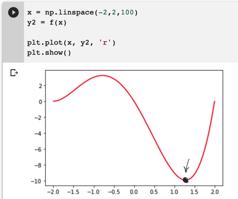
In classical calculus, we deal with functions of variables such as:
[
y = f(x)
]
However, in calculus of variations we deal with functionals, which depend on entire functions.
A common form of a functional is:
[
J[y] = \int_{x_1}^{x_2} F(x, y, y’) dx
]
Here:
- (y(x)) is the function to be determined
- (y’) is its derivative
- (F) is a given function
The goal is to find the function (y(x)) that minimizes or maximizes (J[y]).
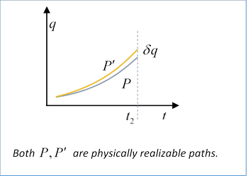
Variations of Functions
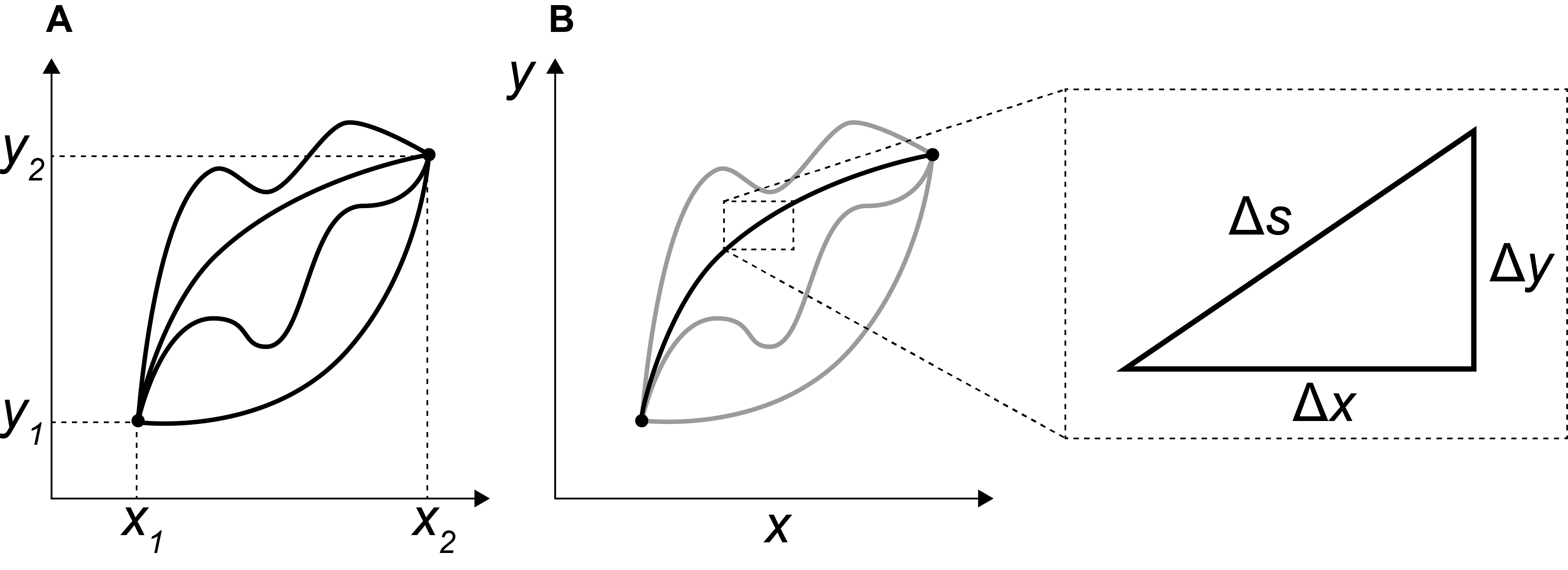
In calculus of variations, we consider small changes in a function called variations.
Suppose a function (y(x)) changes slightly:
[
y(x) \rightarrow y(x) + \epsilon \eta(x)
]
where:
- ( \epsilon ) is a small parameter
- ( \eta(x) ) is a variation function
If the functional is minimized, its first variation must be zero.
This leads to the fundamental equations of variational calculus.
Euler–Lagrange Equation
The central result of the calculus of variations is the Euler–Lagrange equation, which provides the condition for a function to extremize a functional.
genui{“math_block_widget_common_keywords”:{“content”:”\frac{d}{dx}\left(\frac{\partial F}{\partial y’}\right)-\frac{\partial F}{\partial y}=0″}}
This differential equation must be satisfied by the function (y(x)) that makes the functional stationary.
The Euler–Lagrange equation plays a crucial role in many areas of physics and mathematics.
Geometrical Interpretation
The calculus of variations often deals with problems involving curves or surfaces.
For example:
- Shortest path between two points
- Surface area minimization
- Optimal trajectory of a particle
Instead of optimizing numerical values, the goal is to determine the optimal shape of a curve or surface.
The Brachistochrone Problem


The brachistochrone problem is one of the earliest problems solved using variational calculus.
The problem asks:
What curve allows a particle to travel between two points in the shortest time under gravity?
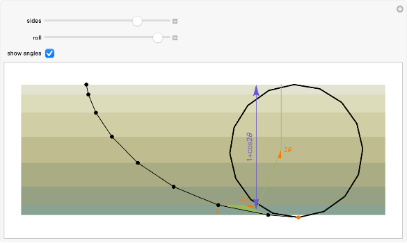
The surprising solution is not a straight line but a cycloid curve.
This problem played an important role in the development of the calculus of variations.
Isoperimetric Problems
Another class of problems studied in variational calculus is isoperimetric problems.
These involve maximizing or minimizing a quantity subject to constraints.
A classic example is:
Among all closed curves with a fixed perimeter, which one encloses the largest area?
The solution is a circle.
Isoperimetric problems lead to the introduction of Lagrange multipliers in variational calculus.
Variational Principles in Physics
One of the most important applications of calculus of variations is in physics.
Many physical laws can be expressed as variational principles.
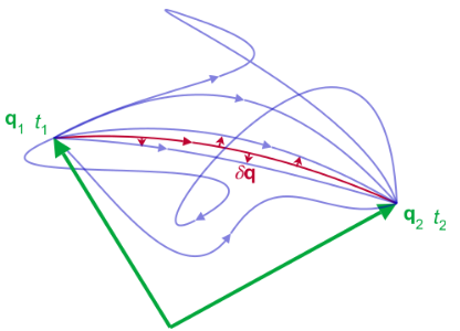
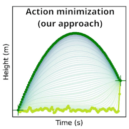
The most famous is the principle of least action.
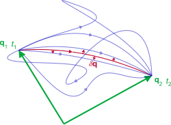
According to this principle, the motion of a system follows a path that minimizes the action functional.
The action is defined as:
[
S = \int L(q,\dot{q},t) dt
]
where:
- (L) is the Lagrangian
- (q) represents generalized coordinates
- (\dot{q}) represents velocities
Applying the Euler–Lagrange equation to the action leads to the equations of motion of the system.
Lagrangian Mechanics
Lagrangian mechanics is a reformulation of classical mechanics based on variational principles.
Instead of forces, the system is described using energy functions.
The Lagrangian is defined as:
[
L = T – V
]
where:
- (T) = kinetic energy
- (V) = potential energy
Using the Euler–Lagrange equation, one can derive the equations of motion for complex systems.
This approach is widely used in physics and engineering.
Hamiltonian Mechanics
The calculus of variations also leads to Hamiltonian mechanics, another formulation of classical mechanics.
The Hamiltonian represents the total energy of the system.
Hamiltonian mechanics is fundamental in:
- Quantum mechanics
- Statistical mechanics
- Dynamical systems
Calculus of Variations in Geometry
Variational methods are widely used in differential geometry.
Examples include:
- Geodesics on curved surfaces
- Minimal surfaces
- Shape optimization problems
Geodesics represent the shortest path between two points on curved surfaces.
Minimal Surfaces


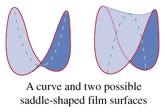
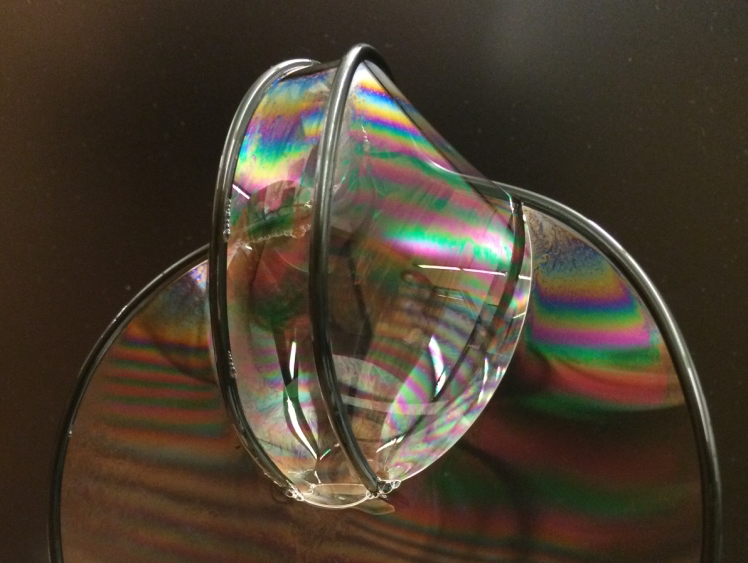
Minimal surfaces are surfaces that minimize surface area.
Soap films provide a physical example.
When a wire frame is dipped into soap solution, the film forms a surface of minimal area.
This phenomenon can be described using calculus of variations.
Applications in Engineering
Calculus of variations has many engineering applications.
Examples include:
- Optimal control systems
- Structural design optimization
- Aerodynamic shape optimization
- Robotics motion planning
Engineers use variational techniques to design efficient systems and structures.
Applications in Economics
Variational methods are also used in economics.
Examples include:
- Optimal resource allocation
- Economic growth models
- Dynamic optimization problems
These models involve maximizing profit or minimizing cost over time.
Numerical Methods in Variational Problems
Many variational problems cannot be solved analytically.
Numerical methods are used to approximate solutions.
Examples include:
- Finite element methods
- Gradient-based optimization
- Dynamic programming
These techniques allow computers to solve complex variational problems.
Modern Developments
Modern research in calculus of variations includes topics such as:
- Optimal control theory
- Variational inequalities
- Nonlinear variational problems
- Applications in machine learning
Variational methods continue to play a central role in modern mathematical research.
Importance in Modern Science
Calculus of variations is fundamental in many scientific disciplines.
It provides a unified framework for describing natural phenomena using optimization principles.
Examples include:
- Physics
- Engineering
- Economics
- Geometry
- Computer science
The concept that nature follows paths of minimum energy or action is central to many scientific theories.
Conclusion
Calculus of variations is a powerful mathematical discipline that focuses on optimizing functionals and determining functions that produce extreme values. Unlike traditional calculus, which deals with functions of variables, variational calculus deals with functionals that depend on entire functions.
The Euler–Lagrange equation provides the fundamental condition for solving variational problems and has widespread applications in mathematics and physics. Many physical laws, including the principle of least action in classical mechanics, are formulated using variational principles.
Applications of calculus of variations extend far beyond theoretical mathematics. It plays an essential role in physics, engineering, economics, geometry, and modern computational science. As technology advances and complex systems become more important, variational methods will continue to be a crucial tool for solving optimization problems across many scientific fields.