

Introduction to Functions
In mathematics, functions are fundamental concepts used to describe relationships between quantities. A function defines a rule that assigns exactly one output value to each input value. Functions are essential in almost every branch of mathematics and play a crucial role in fields such as physics, engineering, economics, computer science, statistics, and many other disciplines.
The concept of a function allows mathematicians and scientists to model real-world relationships. For example, the distance traveled by a car depends on time, temperature may depend on time of day, and the profit of a business may depend on the number of products sold. These relationships can all be represented using functions.
A simple example of a function is:
[
f(x) = x^2
]
In this function, each value of (x) is mapped to a value of (x^2). If (x = 3), then:
[
f(3) = 9
]
This means the output of the function is determined entirely by the input.
Functions help us understand patterns, analyze relationships between variables, and make predictions about future behavior based on known data.
Definition of a Function
A function is a relation between two sets where each element in the first set corresponds to exactly one element in the second set.
The first set is called the domain, and the second set is called the range.
General notation:
[
f: A \rightarrow B
]
This means function (f) maps elements from set (A) to set (B).
Example:
[
f(x) = 2x + 3
]
Here:
Input (x = 2)
[
f(2) = 2(2) + 3 = 7
]
Thus, the function maps the value 2 to 7.
Components of a Function
A function consists of several key components that define how it operates.
Domain
The domain is the set of all possible input values for which the function is defined.
Example:
For function:
[
f(x) = \frac{1}{x}
]
The domain is all real numbers except (x = 0).
Range
The range is the set of all possible output values produced by the function.
Example:
For:
[
f(x) = x^2
]
Range = all non-negative numbers.
Co-domain
The co-domain is the set in which output values lie, though not all values must necessarily appear.
Input and Output
Input is the independent variable, usually (x).
Output is the dependent variable, usually (y).
Function Notation
Functions are usually written using notation such as:
[
f(x)
]
Here:
- (f) is the function name
- (x) is the input
Example:
[
f(x) = x + 4
]
Then:
[
f(5) = 9
]
Other common notations include:
[
g(x), h(x), p(x)
]
Representations of Functions
Functions can be represented in multiple ways.
Algebraic Representation
Using mathematical formulas.
Example:
[
f(x) = x^2 + 3x + 2
]
Graphical Representation
Functions can be plotted on coordinate planes.
The graph of a function consists of points:
[
(x, f(x))
]
Example:
Graph of (y = x^2) is a parabola.
Tabular Representation
Functions can be represented using tables.
Example:
| x | f(x) |
|---|---|
| 1 | 1 |
| 2 | 4 |
| 3 | 9 |
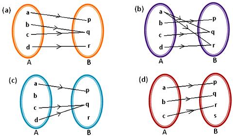
Mapping Diagram
A diagram showing how elements of domain map to elements of range.
Vertical Line Test
To determine whether a graph represents a function, mathematicians use the vertical line test.
Rule:
A graph represents a function if no vertical line intersects the graph more than once.
If a vertical line touches the graph at multiple points, then it is not a function.
Example:
A circle fails the vertical line test.
Types of Functions
Functions come in many forms depending on their mathematical structure.
Constant Function
A constant function always produces the same output.
Example:
[
f(x) = 5
]
Graph is a horizontal line.
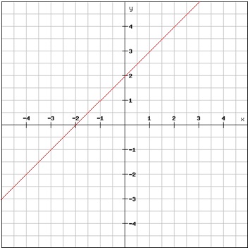
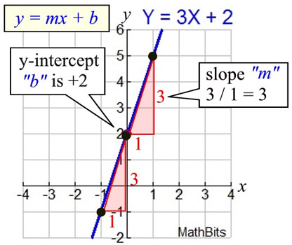
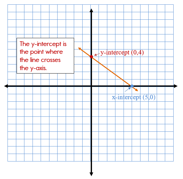
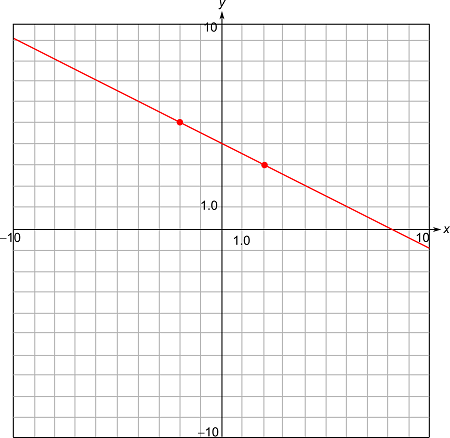
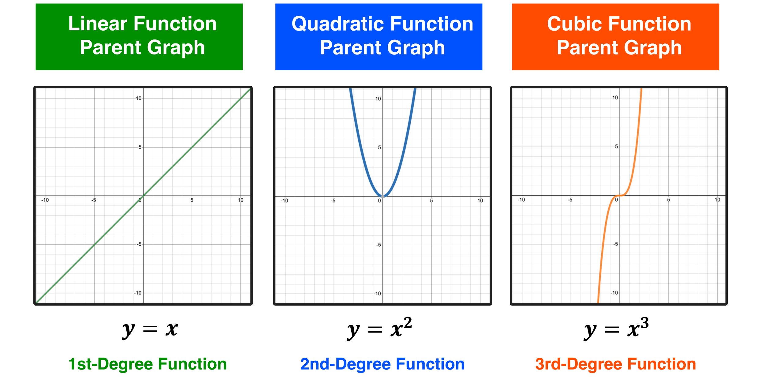
Linear Function
A linear function has the form:
[
f(x) = mx + b
]
Where:
- (m) = slope
- (b) = y-intercept
Example:
[
f(x) = 2x + 1
]
Graph is a straight line.
Quadratic Function
A quadratic function has degree 2.
Example:
[
f(x) = ax^2 + bx + c
]
Graph is a parabola.
Polynomial Function
A polynomial function contains powers of variables.
Example:
[
f(x) = x^3 + 2x^2 + x + 1
]
Rational Function
A rational function is a ratio of two polynomials.
Example:
[
f(x) = \frac{x+1}{x-2}
]
Exponential Function
An exponential function has the form:
[
f(x) = a^x
]
Example:
[
f(x) = 2^x
]
These functions grow rapidly.
Logarithmic Function
Logarithmic functions are inverses of exponential functions.
Example:
[
f(x) = \log(x)
]
Trigonometric Functions
Important functions in mathematics and physics.
Examples:
- sine
- cosine
- tangent
Example:
[
f(x) = \sin x
]
Piecewise Functions
A piecewise function is defined by different formulas in different intervals.
Example:
[
f(x) =
\begin{cases}
x^2 & x < 0 \
x+2 & x \ge 0
\end{cases}
]
Even and Odd Functions
Functions can also be classified based on symmetry.
Even Functions
A function is even if:
[
f(-x) = f(x)
]
Example:
[
f(x) = x^2
]
Graph is symmetric about the y-axis.
Odd Functions
A function is odd if:
[
f(-x) = -f(x)
]
Example:
[
f(x) = x^3
]
Graph is symmetric about the origin.
Increasing and Decreasing Functions
A function may increase or decrease depending on input values.
Increasing Function
If:
[
x_1 < x_2
]
then:
[
f(x_1) < f(x_2)
]
Decreasing Function
If:
[
x_1 < x_2
]
then:
[
f(x_1) > f(x_2)
]
Function Composition
Function composition combines two functions.
Example:
[
f(x) = x+1
]
[
g(x) = x^2
]
Composition:
[
(g \circ f)(x) = g(f(x))
]
[
g(f(x)) = (x+1)^2
]
Inverse Functions
An inverse function reverses the effect of the original function.
Example:
[
f(x) = 2x + 3
]
To find inverse:
[
y = 2x + 3
]
Swap variables:
[
x = 2y + 3
]
Solve:
[
y = \frac{x-3}{2}
]
So:
[
f^{-1}(x) = \frac{x-3}{2}
]
Domain and Range Analysis
Understanding domain and range is essential when analyzing functions.
Example:
[
f(x) = \sqrt{x}
]
Domain:
[
x \ge 0
]
Range:
[
y \ge 0
]
Transformations of Functions
Functions can be transformed in several ways.
Vertical Shift
[
f(x) + c
]
Moves graph up.
Horizontal Shift
[
f(x – c)
]
Moves graph right.
Reflection
Reflection across x-axis:
[
-f(x)
]
Reflection across y-axis:
[
f(-x)
]
Scaling
Vertical stretch:
[
af(x)
]
Horizontal stretch:
[
f(ax)
]
Functions in Calculus
Functions are central to calculus.
Calculus studies:
- Limits
- Derivatives
- Integrals
Example:
Derivative of function describes rate of change.
[
f(x) = x^2
]
Derivative:
[
f'(x) = 2x
]
Applications of Functions
Functions are used extensively in real-world situations.
Physics
Functions describe motion, energy, and force.
Example:
Distance function:
[
d(t) = vt
]
Economics
Functions model cost, revenue, and profit.
Example:
[
Profit = Revenue – Cost
]
Computer Science
Functions appear in algorithms and programming.
Many programming languages implement functions as reusable code blocks.
Engineering
Functions model electrical signals, system responses, and mechanical systems.
Statistics
Probability distributions are functions.
Example:
Normal distribution.
Historical Development of Functions
The concept of function evolved over centuries.
Ancient mathematicians studied relationships between quantities without formal function notation.
In the 17th century, mathematicians like Leibniz introduced the term function.
Later mathematicians such as Euler formalized the concept.
Modern set theory defines functions using mappings between sets.
Importance of Functions in Mathematics
Functions are important because they:
- Describe relationships between variables
- Help model real-world systems
- Provide tools for prediction and analysis
- Serve as foundation for calculus and advanced mathematics
Nearly every branch of mathematics uses functions.
Conclusion
Functions are one of the most powerful and fundamental concepts in mathematics. They allow us to express relationships between quantities and analyze how one variable changes in response to another. Through algebraic expressions, graphs, tables, and mappings, functions provide multiple ways to understand and interpret mathematical relationships.
From simple linear equations to complex exponential and trigonometric models, functions form the backbone of mathematical analysis and scientific modeling. Their applications extend across numerous disciplines including physics, engineering, economics, computer science, and statistics.
Understanding functions enables mathematicians and scientists to explore patterns, solve problems, predict outcomes, and build mathematical models that explain the behavior of the world around us.
Mastery of functions provides the foundation for advanced mathematical topics such as calculus, differential equations, and mathematical modeling, making them an essential topic in the study of mathematics.