Tag Archives: coordinate geometry

Vectors – Detailed Explanation

1. Introduction to Vectors

Vectors are one of the most fundamental concepts in mathematics and physics. They are widely used to represent quantities that have both magnitude and direction. Unlike scalar quantities, which only describe magnitude, vectors capture both size and direction, making them essential in describing motion, forces, displacement, velocity, and many physical phenomena.

The concept of vectors is extensively used in several fields such as mathematics, physics, engineering, computer graphics, navigation, robotics, machine learning, and data science. In geometry and algebra, vectors help describe movement, transformation, and spatial relationships.

A vector can be visually represented as an arrow. The length of the arrow indicates the magnitude of the vector, while the direction of the arrow shows the direction in which the vector acts.

For example:

Distance is a scalar quantity because it only tells how far something has moved.
Displacement is a vector quantity because it tells both the distance and the direction of movement.

If a person walks 5 meters east, the magnitude is 5 meters and the direction is east, forming a vector.

Vectors are usually denoted using bold letters or with an arrow on top of the variable.

Examples:

v⃗ , a⃗ , F⃗

These symbols represent vectors with both magnitude and direction.

Vectors form the foundation of vector algebra and vector calculus, which are essential tools for studying motion, forces, and spatial relationships.

2. Scalar Quantities vs Vector Quantities

To understand vectors clearly, it is important to differentiate between scalar quantities and vector quantities.

Scalar Quantities

Scalar quantities have only magnitude and no direction.

Examples include:

Mass
Temperature
Time
Energy
Speed
Distance
Volume
Density

For instance, if the temperature is 30°C, only the magnitude matters.

Vector Quantities

Vector quantities possess both magnitude and direction.

Examples include:

Displacement
Velocity
Acceleration
Force
Momentum
Electric field
Magnetic field

For example:

Velocity = 20 m/s north

Here,

Magnitude = 20 m/s
Direction = north

3. Representation of Vectors

Vectors can be represented in several ways.

Geometric Representation

Vectors are represented as directed line segments (arrows).

The starting point is called the tail
The ending point is called the head

The arrow shows the direction of the vector.

For example, if vector AB is drawn from point A to point B, it is written as:

AB⃗

The magnitude is represented as:

|AB⃗|

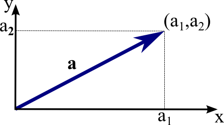
Coordinate Representation

In a Cartesian coordinate system, vectors are expressed using components.

For example:

v = (x, y)

This means the vector moves:

x units in horizontal direction
y units in vertical direction

Example:

v = (3,4)

This means:

3 units in x-direction
4 units in y-direction

The magnitude of this vector is:

|v| = √(3² + 4²)
|v| = √(9 + 16)
|v| = √25
|v| = 5

Column Vector Form

Vectors can also be written in column form:

v =
[ x ]
[ y ]

For example:

v =
[ 3 ]
[ 4 ]

Unit Vector Form

Vectors can be expressed using unit vectors.

In 3D space, three standard unit vectors are used:

i → x direction
j → y direction
k → z direction

A vector can be written as:

v = xi + yj + zk

Example:

v = 3i + 4j

This means:

3 units along x-axis
4 units along y-axis

4. Magnitude of a Vector

The magnitude of a vector represents its length.

For a vector:

v = (x, y)

The magnitude is:

|v| = √(x² + y²)

For a 3D vector:

v = (x, y, z)

Magnitude is:

|v| = √(x² + y² + z²)

Example:

v = (2, 3, 6)

|v| = √(2² + 3² + 6²)
|v| = √(4 + 9 + 36)
|v| = √49
|v| = 7

5. Types of Vectors

Zero Vector

A zero vector has magnitude zero and no direction.

It is represented as:

0⃗

Example:

(0,0)

Unit Vector

A vector with magnitude 1 is called a unit vector.

Example:

i = (1,0)
j = (0,1)

Unit vectors indicate direction.

Equal Vectors

Two vectors are equal if:

Their magnitudes are equal
Their directions are the same

Example:

A = (2,3)
B = (2,3)

Negative Vectors

Negative vectors have the same magnitude but opposite direction.

Example:

A = (3,4)

Negative vector:

−A = (−3,−4)

Parallel Vectors

Vectors pointing in the same or opposite direction.

Example:

A = (2,4)
B = (1,2)

These are parallel because B is a scaled version of A.

Collinear Vectors

Vectors lying on the same straight line are called collinear vectors.

Position Vector

A vector representing the position of a point from the origin.

Example:

Point P(3,4)

Position vector:

OP = (3,4)

6. Vector Addition

Vectors can be added together.

There are two geometric methods:

Triangle Law of Vector Addition

If vector B is placed at the head of vector A, the resultant vector is drawn from the tail of A to the head of B.

Mathematically:

R = A + B

Parallelogram Law

Two vectors are drawn from the same point.

A parallelogram is formed.

The diagonal represents the resultant vector.

Algebraic Addition

If:

A = (x₁,y₁)
B = (x₂,y₂)

Then:

A + B = (x₁ + x₂ , y₁ + y₂)

Example:

A = (2,3)
B = (4,1)

A + B = (6,4)

7. Vector Subtraction

Vector subtraction is defined as:

A − B = A + (−B)

Example:

A = (5,7)
B = (2,3)

A − B = (3,4)

8. Scalar Multiplication of Vectors

A vector can be multiplied by a scalar number.

If:

v = (x,y)

Then:

kv = (kx, ky)

Example:

v = (2,3)

3v = (6,9)

This changes the magnitude but not the direction (unless scalar is negative).

9. Dot Product (Scalar Product)

The dot product of two vectors produces a scalar value.

Formula:

A · B = |A||B| cosθ

Where:

θ = angle between vectors

In component form:

A · B = x₁x₂ + y₁y₂

Example:

A = (2,3)
B = (4,5)

A · B = (2×4) + (3×5)
= 8 + 15
= 23

Properties of Dot Product

A · B = B · A
A · (B + C) = A · B + A · C
A · A = |A|²

Applications of Dot Product

Dot product is used to:

Calculate angles between vectors
Determine orthogonality
Work calculations in physics
Projection of vectors

10. Cross Product (Vector Product)

Cross product results in another vector.

Formula:

A × B = |A||B| sinθ n̂

Where:

n̂ = unit vector perpendicular to both vectors.

In determinant form:

A × B =

| i j k |
| a₁ a₂ a₃ |
| b₁ b₂ b₃ |

Properties

A × B = −(B × A)
A × A = 0
Cross product is perpendicular to both vectors.

Applications

Used in:

Torque calculation
Angular momentum
Magnetic force
3D graphics

11. Vector Projection

Projection of vector A onto vector B:

Proj_B(A) = (A · B / |B|²) B

This represents how much of vector A lies in the direction of B.

12. Direction Cosines

Direction cosines describe the angles a vector makes with coordinate axes.

If a vector makes angles α, β, γ with x, y, z axes:

cosα = x/|v|
cosβ = y/|v|
cosγ = z/|v|

Property:

cos²α + cos²β + cos²γ = 1

13. Vectors in Three Dimensions

In 3D space, vectors have three components.

Example:

v = (x,y,z)

This represents movement in:

x-direction
y-direction
z-direction

Example:

v = (2,4,6)

Magnitude:

|v| = √(2² + 4² + 6²)

14. Applications of Vectors

Vectors are used in many real-world areas.

Physics

Vectors describe motion, forces, and acceleration.

Examples:

Newton’s laws
Electromagnetism
Fluid dynamics

Engineering

Vectors help analyze structures and forces.

Examples:

Structural engineering
Mechanical systems
Robotics

Computer Graphics

Vectors are used to represent:

3D models
Lighting
Motion

Game engines rely heavily on vector calculations.

Navigation

Vectors are used to determine:

Direction
Distance
Movement

Aircraft and ships use vector navigation.

Machine Learning

Vectors represent data points in multi-dimensional space.

Example:

Feature vectors in AI models.

15. Vectors in Geometry

Vectors simplify geometry calculations.

Applications include:

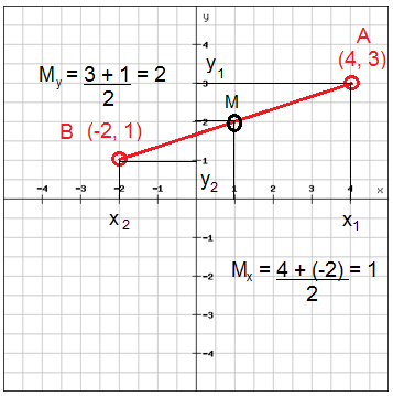
Distance between points
Midpoint calculation
Area of triangles
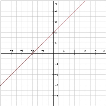
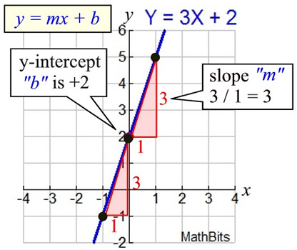
Equation of lines

Example:

Distance formula using vectors.

16. Linear Combination of Vectors

A vector can be expressed as a combination of other vectors.

Example:

v = aA + bB

Where a and b are scalars.

17. Linear Independence

Vectors are linearly independent if none can be written as a combination of the others.

This concept is important in:

Linear algebra
Matrix theory
Vector spaces

18. Vector Spaces

A vector space is a collection of vectors satisfying certain rules.

Properties include:

Closure under addition
Closure under scalar multiplication
Existence of zero vector
Existence of inverse vectors

Examples:

R² space
R³ space
Polynomial vector spaces

19. Basis and Dimension

A basis is a set of vectors that can generate the entire vector space.

Example:

In 2D space:

i = (1,0)
j = (0,1)

Dimension is the number of basis vectors.

2D → dimension = 2
3D → dimension = 3

20. Importance of Vectors

Vectors are essential because they provide a powerful way to represent spatial relationships.

They allow:

Efficient representation of motion
Simplification of geometric problems
Modeling of physical systems
Data representation in machine learning

Without vectors, many modern technologies such as computer graphics, robotics, and artificial intelligence would not be possible.

Conclusion

Vectors are fundamental mathematical objects used to describe quantities with both magnitude and direction. They play a critical role in mathematics, physics, engineering, computer science, and many modern technological fields. From representing motion in physics to powering algorithms in artificial intelligence, vectors provide a structured way to model real-world phenomena.

Understanding vectors includes learning how to represent them, perform operations such as addition and multiplication, and apply them in various contexts. Concepts like dot product, cross product, vector spaces, and linear independence form the basis of advanced mathematical studies.

Because vectors describe direction and magnitude simultaneously, they serve as an essential bridge between geometry and algebra. Their applications extend far beyond theoretical mathematics and are deeply embedded in modern science and technology.

Coordinate Geometry

Introduction to Coordinate Geometry

Coordinate geometry, also known as analytic geometry, is a branch of mathematics that combines algebra and geometry to study geometric figures using a coordinate system. In this system, points are represented by numerical coordinates that describe their position in a plane.

The development of coordinate geometry revolutionized mathematics by allowing geometric problems to be solved using algebraic equations. This approach makes it easier to analyze shapes, calculate distances, determine slopes, and represent curves.

Coordinate geometry is widely used in mathematics, physics, engineering, computer science, navigation, and many other scientific fields. It provides a powerful framework for understanding spatial relationships and solving problems involving geometric figures.

The most common coordinate system used in coordinate geometry is the Cartesian coordinate system, which uses two perpendicular axes to locate points in a plane.

Historical Background

Coordinate geometry was developed in the 17th century by the French mathematician René Descartes. His work established a method of representing geometric shapes using algebraic equations.

Before Descartes introduced this concept, geometry and algebra were treated as separate branches of mathematics. By combining them, Descartes created a powerful mathematical tool that allowed curves and shapes to be analyzed using equations.

The Cartesian coordinate system was named after Descartes in recognition of his contribution to mathematics.

Cartesian Coordinate System

The Cartesian coordinate system consists of two perpendicular number lines called axes.

These axes intersect at a point called the origin.

The horizontal axis is called the x-axis.

The vertical axis is called the y-axis.

The point where the axes intersect is represented as:

[
(0,0)
]

This point is called the origin.

Axes of the Coordinate Plane

The coordinate plane consists of two axes.

X-axis

The x-axis is the horizontal axis.

It represents horizontal movement across the plane.

Y-axis

The y-axis is the vertical axis.

It represents vertical movement.

Coordinates of a Point

Every point in the coordinate plane is represented by an ordered pair.

The ordered pair is written as:

[
(x,y)
]

Where:

(x) is the horizontal coordinate
(y) is the vertical coordinate

Example:

[
(3,4)
]

This means the point lies:

3 units along the x-axis
4 units along the y-axis

Quadrants of the Coordinate Plane

The coordinate plane is divided into four regions called quadrants.

First Quadrant

Both coordinates are positive.

[
(+,+)
]

Example:

(4,5)

Second Quadrant

x is negative, y is positive.

[
(-,+)
]

Example:

(-3,4)

Third Quadrant

Both coordinates are negative.

[
(-,-)
]

Example:

(-5,-2)

Fourth Quadrant

x is positive, y is negative.

[
(+,-)
]

Example:

(4,-3)

Plotting Points

Plotting points involves locating coordinates on the plane.

Steps:

Start at the origin.
Move along the x-axis according to the x-value.
Move vertically according to the y-value.
Mark the point.

Example:

Point (2,3)

Move 2 units right, then 3 units up.

Distance Between Two Points

One of the most important formulas in coordinate geometry is the distance formula.

For two points:

[
(x_1,y_1) \quad and \quad (x_2,y_2)
]

Distance:

[
d = \sqrt{(x_2-x_1)^2 + (y_2-y_1)^2}
]

This formula is derived from the Pythagorean theorem.

Example of Distance Formula

Points:

[
(1,2) \quad and \quad (4,6)
]

Distance:

[
d = \sqrt{(4-1)^2 + (6-2)^2}
]

[
d = \sqrt{9 + 16}
]

[
d = \sqrt{25}
]

[
d = 5
]

Midpoint Formula

The midpoint of a line segment is the point that divides the segment into two equal parts.

Formula:

[
M = \left(\frac{x_1+x_2}{2}, \frac{y_1+y_2}{2}\right)
]

Example of Midpoint

Points:

[
(2,4) \quad and \quad (6,8)
]

Midpoint:

[
M = (4,6)
]

Slope of a Line

The slope measures how steep a line is.

Formula:

[
m = \frac{y_2 – y_1}{x_2 – x_1}
]

Slope represents the rate of change between two points.

Types of Slopes

Lines can have different types of slopes.

Positive Slope

Line rises from left to right.

Example:

(m > 0)

Negative Slope

Line falls from left to right.

Example:

(m < 0)

Zero Slope

Horizontal line.

Example:

(m = 0)

Undefined Slope

Vertical line.

Division by zero occurs.

Equation of a Line

Lines in coordinate geometry are represented by equations.

Slope-Intercept Form

[
y = mx + c
]

Where:

(m) = slope
(c) = y-intercept

Example

[
y = 2x + 3
]

Slope = 2
Y-intercept = 3

Point-Slope Form

[
y – y_1 = m(x – x_1)
]

Used when slope and one point are known.

Two-Point Form

Used when two points are known.

[
y-y_1 = \frac{y_2-y_1}{x_2-x_1}(x-x_1)
]

Intercept Form

[
\frac{x}{a} + \frac{y}{b} = 1
]

Where:

(a) = x-intercept
(b) = y-intercept

Parallel Lines

Two lines are parallel if they have the same slope.

Example:

[
y = 3x + 1
]

[
y = 3x – 4
]

Both have slope 3.

Perpendicular Lines

Two lines are perpendicular if the product of their slopes equals -1.

Example:

If:

[
m_1 = 2
]

Then:

[
m_2 = -\frac{1}{2}
]

Area of Triangle in Coordinate Geometry

Area formula using coordinates:

[
A = \frac{1}{2} |x_1(y_2-y_3)+x_2(y_3-y_1)+x_3(y_1-y_2)|
]

Equation of a Circle

Circle equation in coordinate geometry:

[
(x-h)^2 + (y-k)^2 = r^2
]

Where:

(h,k) = center
r = radius

Graphs of Functions

Coordinate geometry allows functions to be represented graphically.

Example:

[
y = x^2
]

This produces a parabola.

Transformations in Coordinate Geometry

Graphs can be transformed by shifting, stretching, or reflecting.

Example:

[
y = (x-2)^2
]

Shifted right by 2 units.

Applications of Coordinate Geometry

Coordinate geometry has many practical applications.

Engineering

Used in structural design and mechanical systems.

Physics

Used to analyze motion and forces.

Computer Graphics

Digital images and animations rely heavily on coordinate geometry.

Navigation

GPS systems use coordinates to determine location.

Robotics

Robot movements are calculated using coordinate systems.

Architecture

Building layouts are designed using coordinate-based plans.

Coordinate Geometry in Calculus

In calculus, coordinate geometry helps analyze curves.

Concepts include:

derivatives
integrals
limits

Curves are described using equations in the coordinate plane.

Three-Dimensional Coordinate Geometry

Beyond two dimensions, coordinate systems extend into 3D space.

Coordinates are written as:

[
(x,y,z)
]

Axes include:

x-axis
y-axis
z-axis

Used in physics, engineering, and computer graphics.

Importance of Coordinate Geometry

Coordinate geometry is important because it:

connects algebra and geometry
simplifies geometric calculations
allows precise representation of shapes
supports advanced mathematics

It forms the basis for many modern technologies.

Conclusion

Coordinate geometry is a powerful branch of mathematics that combines algebraic techniques with geometric concepts to study shapes and relationships in a coordinate plane. By representing points as ordered pairs and using equations to describe lines and curves, coordinate geometry allows mathematicians and scientists to analyze spatial relationships with precision.

From calculating distances and slopes to graphing equations and studying geometric figures, coordinate geometry provides essential tools for solving mathematical problems. Its applications extend far beyond mathematics into fields such as physics, engineering, computer graphics, navigation, and robotics.

Understanding coordinate geometry lays the foundation for advanced mathematical topics such as calculus, linear algebra, and analytical geometry, making it one of the most important areas of mathematical study.

Linear Equations in Mathematics

Linear equations are one of the most fundamental topics in algebra and mathematics. They represent relationships between variables that form straight-line graphs when plotted on a coordinate plane. Linear equations are widely used in mathematics, physics, economics, engineering, computer science, and many other scientific disciplines.

A linear equation is an equation in which the highest power of the variable is one. This means the variables are not squared, cubed, or raised to higher powers. Linear equations describe relationships that change at a constant rate.

For example:

2x + 3 = 7

This equation contains a variable x, constants 2, 3, and 7, and the equation shows a relationship that can be solved to find the value of x.

Linear equations are essential because they form the basis for understanding more advanced mathematical concepts such as systems of equations, matrices, calculus, and mathematical modeling.

1. Definition of a Linear Equation

A linear equation is an algebraic equation in which each variable has an exponent of one, and the equation forms a straight line when graphed.

General form:

ax + b = 0

Where:

a and b are constants
x is a variable

Example:

3x + 5 = 11

Here:

3 is the coefficient
5 is the constant term
x is the variable

Linear equations are called “linear” because they produce linear graphs (straight lines).

2. Components of a Linear Equation

Linear equations contain several key components.

Variables

Variables represent unknown values.

Example:

x, y, z

Example equation:

2x + 4 = 10

Here x is the variable.

Constants

Constants are fixed numbers.

Example:

In the equation:

3x + 7 = 16

The numbers 7 and 16 are constants.

Coefficients

A coefficient is a number multiplied by a variable.

Example:

Here 5 is the coefficient.

Terms

Terms are parts of an equation separated by addition or subtraction.

Example:

4x + 6

Terms:

4x and 6

3. Types of Linear Equations

Linear equations can appear in several different forms.

Linear Equation in One Variable

These equations contain only one variable.

Example:

5x + 3 = 13

Solution:

5x = 10

x = 2

Linear Equation in Two Variables

These equations contain two variables.

Example:

2x + y = 6

Solutions include pairs of numbers that satisfy the equation.

Example:

x = 2, y = 2

Linear Equation in Three Variables

Example:

x + y + z = 6

These equations are used in advanced algebra and linear systems.

4. Standard Form of Linear Equation

The standard form of a linear equation in two variables is:

Ax + By + C = 0

Where:

A, B, and C are constants
A and B are not both zero

Example:

2x + 3y − 6 = 0

This form is useful in coordinate geometry.

5. Slope-Intercept Form

Another important form is:

y = mx + b

Where:

m is the slope
b is the y-intercept

Example:

y = 2x + 3

Slope = 2
Intercept = 3

This means the line crosses the y-axis at 3.

6. Graph of Linear Equations

A linear equation in two variables represents a straight line on a coordinate plane.

Steps to graph a linear equation:

Convert equation into slope-intercept form.
Identify slope and intercept.
Plot the intercept.
Use the slope to find additional points.
Draw a straight line through the points.

Example:

y = x + 2

Points:

(0,2)

(1,3)

(2,4)

These points form a straight line.

7. Solving Linear Equations

Solving a linear equation means finding the value of the variable.

Example 1

3x + 5 = 11

Step 1:

Subtract 5

3x = 6

Step 2:

Divide by 3

x = 2

Example 2

5x − 4 = 16

Add 4:

5x = 20

Divide by 5:

x = 4

8. Linear Equations with Variables on Both Sides

Example:

2x + 5 = x + 9

Step 1:

Subtract x from both sides

x + 5 = 9

Step 2:

Subtract 5

x = 4

9. Systems of Linear Equations

A system of linear equations contains two or more equations with the same variables.

Example:

x + y = 5
x − y = 1

The solution is the point where both equations are satisfied.

10. Methods for Solving Systems

Substitution Method

Solve one equation for a variable and substitute into the other.

Example:

x = 5 − y

Substitute into the second equation.

Elimination Method

Add or subtract equations to eliminate a variable.

Example:

x + y = 5
x − y = 1

Add equations:

2x = 6

x = 3

Substitute:

y = 2

Graphical Method

Plot both equations on a graph.

The intersection point is the solution.

11. Special Cases of Linear Systems

Systems may have:

One Solution

Lines intersect at one point.

Infinite Solutions

Lines overlap completely.

No Solution

Lines are parallel.

12. Linear Equations in Real-Life Applications

Linear equations appear in many practical situations.

Economics

Profit equations:

Profit = Revenue − Cost

Physics

Motion equation:

distance = speed × time

Business

Cost calculations:

Total cost = fixed cost + variable cost

Engineering

Linear models describe relationships between variables.

13. Linear Functions

A linear function describes a relationship between variables.

Example:

f(x) = 3x + 2

This function produces a straight line graph.

Linear functions describe constant rates of change.

14. Linear Equations in Coordinate Geometry

Linear equations represent lines on a coordinate plane.

Key concepts include:

slope
intercepts
parallel lines
perpendicular lines

Parallel Lines

Parallel lines have the same slope.

Example:

y = 2x + 3
y = 2x − 4

Perpendicular Lines

Perpendicular lines have slopes that are negative reciprocals.

Example:

Slope = 2

Perpendicular slope = −1/2

15. Linear Equations in Matrices

In higher mathematics, systems of linear equations can be represented using matrices.

Example:

AX = B

Matrix methods help solve large systems efficiently.

16. Importance of Linear Equations

Linear equations are essential because they:

describe relationships between variables
model real-world problems
provide a foundation for algebra

They are used extensively in science and technology.

17. Linear Equations in Computer Science

In computing, linear equations appear in:

machine learning
optimization algorithms
graphics transformations

Many algorithms rely on solving systems of linear equations.

18. Historical Development of Linear Algebra

The study of linear equations dates back to ancient civilizations.

Chinese mathematicians used methods similar to modern matrix techniques to solve systems of equations.

These ideas later developed into modern algebra and linear algebra.

19. Advanced Concepts Related to Linear Equations

Advanced topics include:

linear programming
vector spaces
matrix algebra
numerical methods

These topics extend the study of linear relationships.

20. Summary

Linear equations are fundamental mathematical expressions that represent relationships between variables where the highest exponent is one. These equations form straight lines when graphed and describe constant rates of change.

They are essential tools in algebra and are widely used in science, economics, engineering, and computer science. Understanding linear equations involves learning their forms, solving methods, graphical interpretation, and real-world applications.

Mastery of linear equations provides a strong foundation for advanced mathematics and problem-solving in many fields.

1. Introduction to Vectors

2. Scalar Quantities vs Vector Quantities

Scalar Quantities

Vector Quantities

3. Representation of Vectors

Geometric Representation

Coordinate Representation

Column Vector Form

Unit Vector Form

4. Magnitude of a Vector

5. Types of Vectors

Zero Vector

Unit Vector

Equal Vectors

Negative Vectors

Parallel Vectors

Collinear Vectors

Position Vector

6. Vector Addition

Triangle Law of Vector Addition

Parallelogram Law

Algebraic Addition

7. Vector Subtraction

8. Scalar Multiplication of Vectors

9. Dot Product (Scalar Product)

Properties of Dot Product

Applications of Dot Product

10. Cross Product (Vector Product)

Properties

Applications

11. Vector Projection

12. Direction Cosines

13. Vectors in Three Dimensions

14. Applications of Vectors

Physics

Engineering

Computer Graphics

Navigation

Machine Learning

15. Vectors in Geometry

16. Linear Combination of Vectors

17. Linear Independence

18. Vector Spaces

19. Basis and Dimension

20. Importance of Vectors

Conclusion

Tags

Introduction to Coordinate Geometry

Historical Background

Cartesian Coordinate System

Axes of the Coordinate Plane

X-axis

Y-axis

Coordinates of a Point

Quadrants of the Coordinate Plane

First Quadrant

Second Quadrant

Third Quadrant

Fourth Quadrant

Plotting Points

Distance Between Two Points

Example of Distance Formula

Midpoint Formula

Example of Midpoint

Slope of a Line

Types of Slopes

Positive Slope

Negative Slope

Zero Slope

Undefined Slope

Equation of a Line

Slope-Intercept Form

Example

Point-Slope Form

Two-Point Form

Intercept Form

Parallel Lines

Perpendicular Lines

Area of Triangle in Coordinate Geometry

Equation of a Circle