Tag Archives: Mathematical Functions

Polynomials — A Complete Guide in Mathematics

Image
Image
Image

Introduction to Polynomials

In mathematics, polynomials are one of the most fundamental and widely used algebraic structures. They appear in algebra, calculus, number theory, engineering, economics, physics, computer science, and many other fields. A polynomial is an algebraic expression composed of variables, constants, and exponents combined using addition, subtraction, and multiplication.

Unlike many other mathematical expressions, polynomials do not include variables in denominators, negative exponents, fractional exponents, or radicals involving variables. Because of this restriction, polynomials are relatively easy to analyze and manipulate, making them essential building blocks in mathematics.

A simple example of a polynomial is:

[
3x^2 + 2x + 5
]

In this expression:

  • 3x² is a term
  • 2x is another term
  • 5 is the constant term

Together they form a polynomial expression.

Polynomials are important because they can approximate complex functions, describe curves and surfaces, represent physical phenomena, and solve real-world problems.


Definition of Polynomial

A polynomial is an expression of the form:

[
a_n x^n + a_{n-1} x^{n-1} + \dots + a_2 x^2 + a_1 x + a_0
]

Where:

  • x = variable
  • a₀, a₁, a₂ … aₙ = constants called coefficients
  • n = non-negative integer (degree of polynomial)

Example:

[
4x^3 + 2x^2 – 7x + 9
]

Here:

  • Degree = 3
  • Coefficients = 4, 2, -7
  • Constant = 9

Components of a Polynomial

A polynomial consists of several important parts.

1. Terms

A term is a single part of a polynomial separated by addition or subtraction.

Example:

[
5x^3 + 2x^2 – 4x + 7
]

Terms are:

  • 5x³
  • 2x²
  • -4x
  • 7

2. Coefficient

The coefficient is the numerical factor multiplied by the variable.

Example:

In 6x², the coefficient is 6.


3. Constant

The constant term has no variable.

Example:

[
4x^3 + 5x – 8
]

Constant = -8


4. Degree

The degree of a polynomial is the highest exponent of the variable.

Example:

[
7x^4 + 3x^2 + x + 1
]

Degree = 4


Types of Polynomials Based on Number of Terms

Polynomials can be classified based on how many terms they contain.

Monomial

A polynomial with one term.

Examples:

[
5x^2
]

[
7y
]

[
3
]


Binomial

A polynomial with two terms.

Examples:

[
x + 5
]

[
3x^2 – 7
]


Trinomial

A polynomial with three terms.

Examples:

[
x^2 + 3x + 5
]

[
2x^2 – x + 7
]


Polynomial (General)

A polynomial with more than three terms.

Example:

[
x^4 + 2x^3 + 3x^2 + x + 6
]


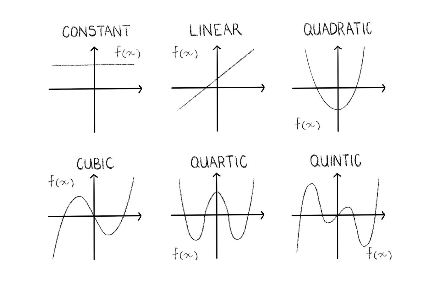
Types of Polynomials Based on Degree

Polynomials are also classified by degree.

Constant Polynomial

Degree = 0

Example:

[
7
]


Linear Polynomial

Degree = 1

Example:

[
2x + 3
]

Graph of a linear polynomial is a straight line.


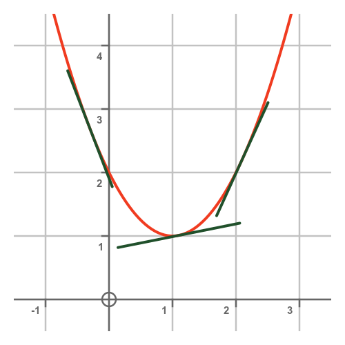
Quadratic Polynomial

Degree = 2

Example:

[
x^2 + 3x + 2
]

Graph is a parabola.


Cubic Polynomial

Degree = 3

Example:

[
x^3 + 2x^2 – x + 5
]

Graph can have up to two turning points.


Quartic Polynomial

Degree = 4

Example:

[
x^4 + 2x^2 + 1
]

Graph can have three turning points.


Quintic Polynomial

Degree = 5

Example:

[
x^5 + 2x^3 + x + 7
]

Higher degree polynomials have more complex curves.


Polynomial Functions

A polynomial function is a function defined by a polynomial expression.

Example:

[
f(x) = 2x^3 – x + 5
]

This function maps values of x to values of f(x).

Polynomial functions are continuous and smooth.

Properties:

  • No sharp corners
  • No breaks
  • No vertical asymptotes

Operations on Polynomials

Polynomials can be manipulated using various algebraic operations.


Addition of Polynomials

Add like terms.

Example:

[
(3x^2 + 2x + 5) + (2x^2 + 4x + 1)
]

Result:

[
5x^2 + 6x + 6
]


Subtraction of Polynomials

Example:

[
(5x^2 + 4x + 3) – (2x^2 + x + 1)
]

Result:

[
3x^2 + 3x + 2
]


Multiplication of Polynomials

Example:

[
(x + 2)(x + 3)
]

Using distributive property:

[
x^2 + 5x + 6
]


Division of Polynomials

Division methods include:

  • Long division
  • Synthetic division

Example:

[
(x^2 + 5x + 6) ÷ (x + 2)
]

Result:

[
x + 3
]


Factoring Polynomials

Factoring means writing a polynomial as a product of simpler polynomials.

Example:

[
x^2 + 5x + 6
]

Factor:

[
(x + 2)(x + 3)
]

Common factoring methods:

  • Greatest Common Factor (GCF)
  • Factoring trinomials
  • Difference of squares
  • Sum and difference of cubes
  • Grouping

Polynomial Graphs

The graph of a polynomial shows how the function behaves.

Key features:

Intercepts

  • x-intercept → where graph crosses x-axis
  • y-intercept → where graph crosses y-axis

End Behavior

End behavior depends on:

  • Degree
  • Leading coefficient

Example:

If degree is even and coefficient positive:

Graph opens upwards on both sides.
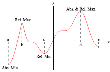

Turning Points

A polynomial of degree n can have at most:

[
n-1
]

turning points.


Polynomial Roots and Zeros

A root or zero of a polynomial is the value of x where:

[
f(x) = 0
]

Example:

[
x^2 – 5x + 6 = 0
]

Factor:

[
(x-2)(x-3)=0
]

Roots:

[
x = 2, 3
]


Fundamental Theorem of Algebra

The Fundamental Theorem of Algebra states:

Every polynomial equation of degree n has exactly n complex roots (counting multiplicity).

Example:

A cubic polynomial always has 3 roots.


Polynomial Theorems

Important theorems related to polynomials include:

Remainder Theorem

If polynomial f(x) is divided by (x − a), remainder is:

[
f(a)
]


Factor Theorem

If:

[
f(a) = 0
]

then (x − a) is a factor.


Applications of Polynomials

Polynomials are widely used in real-world applications.

Physics

Used to describe motion, trajectories, and physical systems.

Example:

Projectile motion equations.


Engineering

Used in:

  • Structural design
  • Signal processing
  • Control systems

Economics

Used to model:

  • Cost functions
  • Revenue functions
  • Profit functions

Computer Graphics

Curves in animation and design often use polynomial interpolation.

Example:

Bezier curves.


Statistics

Regression models use polynomial equations to fit data.


Polynomial Interpolation

Polynomial interpolation is used to find a polynomial that passes through given data points.

Example:

Given points:

(1,2), (2,3), (3,5)

A polynomial can be created that fits these points exactly.

Methods include:

  • Lagrange interpolation
  • Newton interpolation

Special Polynomials

Several special polynomials are important in mathematics.

Chebyshev Polynomials

Used in approximation theory.


Legendre Polynomials

Used in physics, especially in solving differential equations.


Hermite Polynomials

Used in probability theory and quantum mechanics.


Taylor Polynomials

Used in calculus to approximate functions.

Example:

[
e^x \approx 1 + x + x^2/2 + x^3/6
]


Multivariable Polynomials

Polynomials can have more than one variable.

Example:

[
3x^2y + 2xy^2 + 5
]

Variables:

x and y.

These are used in:

  • algebraic geometry
  • optimization
  • physics

Polynomial Rings

In abstract algebra, polynomials form a ring.

Example:

R[x]

This means polynomials with coefficients in ring R.

Polynomial rings are fundamental in:

  • algebra
  • coding theory
  • cryptography

Polynomial Approximation

Many complicated functions can be approximated using polynomials.

Example:

[
sin(x)
]

can be approximated using Taylor polynomial.

This concept is heavily used in:

  • numerical analysis
  • machine learning
  • scientific computing

Advantages of Polynomials

Polynomials are extremely useful because they:

  • Are easy to compute
  • Are continuous and smooth
  • Can approximate many functions
  • Are simple to differentiate and integrate

Limitations of Polynomials

Polynomials cannot represent:

  • Vertical asymptotes
  • Discontinuous functions
  • Exponential growth perfectly
  • Periodic behavior accurately over large intervals

Historical Development of Polynomials

The concept of polynomials has existed for thousands of years.

Ancient Civilizations

Babylonians solved quadratic equations around 2000 BCE.


Greek Mathematics

Greek mathematicians studied geometric interpretations of algebraic equations.


Islamic Golden Age

Persian mathematician Al-Khwarizmi developed systematic algebraic methods.


Renaissance Period

Italian mathematicians discovered formulas for solving cubic and quartic equations.


Modern Mathematics

Polynomials became central in algebra and calculus development.


Polynomials in Modern Technology

Polynomials are used in modern technologies including:

  • Computer graphics
  • Cryptography
  • Signal processing
  • Machine learning algorithms
  • Data fitting
  • Robotics motion planning

Conclusion

Polynomials are among the most important structures in mathematics. Their simplicity, flexibility, and powerful properties make them essential tools for both theoretical mathematics and practical applications.

From basic algebra taught in schools to advanced scientific research, polynomials play a crucial role in understanding patterns, solving equations, modeling real-world systems, and building modern technology.

Their ability to approximate complex functions, describe curves and shapes, and solve practical problems ensures that polynomials remain a central topic in mathematics and science.


Tags

Calculus in Mathematics – Detailed Explanation with Examples

Calculus in Mathematics – Detailed Explanation with Examples

1. Introduction to Calculus

Image
Image
Image
Image

Calculus is one of the most important branches of mathematics that studies change and motion. It focuses on how quantities vary continuously and how we can measure these changes precisely. Calculus is widely used in fields such as physics, engineering, economics, computer science, astronomy, and biology.

The term calculus comes from a Latin word meaning “small stone,” referring to the stones once used for counting and calculations.

Calculus primarily deals with two major concepts:

  1. Differential Calculus – the study of rates of change and slopes of curves.
  2. Integral Calculus – the study of accumulation of quantities and the area under curves.

These two branches are closely related through the Fundamental Theorem of Calculus, which shows how differentiation and integration are inverse processes.

Calculus allows us to answer questions such as:

  • How fast is an object moving at a particular moment?
  • How can we calculate the area under an irregular curve?
  • How do populations grow over time?
  • How can engineers optimize designs?

Before calculus was developed, mathematics mainly dealt with static quantities. Calculus introduced the ability to analyze dynamic systems where values change continuously.


2. Historical Development of Calculus

Image
Image
Image
Image

The development of calculus was a gradual process that involved contributions from many mathematicians.

Early Foundations

Ancient mathematicians studied problems related to area, volume, and motion long before calculus formally existed.

Greek mathematician Archimedes used a technique called the method of exhaustion to calculate areas and volumes of shapes. This method involved approximating a shape using smaller and smaller pieces, which resembles modern integral calculus.

Development in the 17th Century

Calculus was independently developed in the late 17th century by two mathematicians:

  • Isaac Newton
  • Gottfried Wilhelm Leibniz

Newton developed calculus to study motion and physics, especially for understanding planetary movement and gravitational forces.

Leibniz developed a systematic mathematical notation that is still widely used today. His symbols for derivatives and integrals made calculus easier to apply and understand.

Although both mathematicians developed calculus independently, their work together formed the foundation of modern calculus.

Growth of Calculus

After Newton and Leibniz, many mathematicians expanded calculus, including:

  • Euler
  • Lagrange
  • Cauchy
  • Gauss

These mathematicians improved mathematical rigor and developed new techniques for solving complex problems.

Today calculus is a core subject in advanced mathematics and science.


3. Limits – The Foundation of Calculus

Image
Image
Image
Image

The concept of limits is fundamental to calculus.

A limit describes the value that a function approaches as the input approaches a certain number.

For example:

[
\lim_{x \to a} f(x)
]

This means the value that the function f(x) approaches as x approaches a.

Limits allow mathematicians to analyze behavior near a point even if the function is not defined exactly at that point.

Example of a Limit

Consider the function:

[
f(x)=\frac{x^2-1}{x-1}
]

If we substitute x = 1, we get:

[
\frac{1-1}{0}
]

which is undefined.

However, if we simplify:

[
f(x)=x+1
]

Then as x approaches 1, the value approaches 2.

So the limit is:

[
\lim_{x \to 1} \frac{x^2-1}{x-1} = 2
]

Limits help define both derivatives and integrals, making them essential in calculus.


4. Differential Calculus

Image
Image
Image
Image

Differential calculus studies how functions change. It focuses on the rate of change of a quantity.

The central concept in differential calculus is the derivative.

Derivative

The derivative measures how fast a function changes with respect to its variable.

Mathematically:

[
f'(x) = \lim_{h \to 0} \frac{f(x+h)-f(x)}{h}
]

This expression represents the slope of the tangent line to a curve at a specific point.

Geometric Meaning

The derivative represents the slope of a curve at a point.

If a function represents position, its derivative represents velocity.

Example

Given:

[
f(x)=x^2
]

Derivative:

[
f'(x)=2x
]

This means the rate of change of the function increases as x increases.


5. Rules of Differentiation

Differentiation has several rules that simplify calculations.

Power Rule

[
\frac{d}{dx}(x^n)=nx^{n-1}
]

Example:

[
\frac{d}{dx}(x^4)=4x^3
]

Sum Rule

[
\frac{d}{dx}(f(x)+g(x))=f'(x)+g'(x)
]

Product Rule

[
\frac{d}{dx}(uv)=u’v+uv’
]

Quotient Rule

[
\frac{d}{dx}\left(\frac{u}{v}\right)=\frac{u’v-uv’}{v^2}
]

Chain Rule

Used for composite functions.

[
\frac{d}{dx}f(g(x))=f'(g(x))g'(x)
]

These rules allow derivatives of complex functions to be calculated efficiently.


6. Applications of Derivatives

Image
Image
Image
Image

Derivatives have many practical applications.

1. Finding Slopes

Derivatives determine the slope of curves at any point.

2. Velocity and Acceleration

If:

[
s(t)
]

represents position, then:

Velocity:

[
v(t)=\frac{ds}{dt}
]

Acceleration:

[
a(t)=\frac{d^2s}{dt^2}
]

3. Optimization

Derivatives help find maximum and minimum values of functions.

Examples include:

  • Maximizing profit
  • Minimizing cost
  • Designing efficient structures

4. Curve Sketching

Derivatives help analyze:

  • Increasing or decreasing intervals
  • Turning points
  • Concavity

7. Integral Calculus

Image
Image
Image

Integral calculus deals with accumulation and total quantities.

Integration is the reverse process of differentiation.

Indefinite Integral

[
\int f(x)dx
]

This represents the family of functions whose derivative is f(x).

Example:

[
\int 2x,dx=x^2+C
]

where C is a constant.

Definite Integral

[
\int_a^b f(x)dx
]

This calculates the area under the curve between a and b.

Example:

[
\int_0^2 x,dx
]

Solution:

[
\frac{x^2}{2}\Big|_0^2
]

[
=2
]


8. Methods of Integration

Substitution Method

Used when an integral contains a composite function.

Example:

[
\int 2x(x^2+1)^3 dx
]

Let:

[
u=x^2+1
]

Integration by Parts

Formula:

[
\int u,dv=uv-\int v,du
]

Partial Fractions

Used for rational functions.

Trigonometric Integrals

Used when integrals involve sine, cosine, or tangent functions.


9. Fundamental Theorem of Calculus

Image
Image
Image

The Fundamental Theorem of Calculus connects differentiation and integration.

It states that:

If:

[
F(x)=\int_a^x f(t)dt
]

then:

[
F'(x)=f(x)
]

This means:

Differentiation and integration cancel each other.

This theorem makes it possible to evaluate definite integrals using antiderivatives.


10. Applications of Integrals

Image
Image
Image
Image

Integrals have many real-world applications.

1. Area Under Curves

Integrals calculate areas of irregular shapes.

2. Volumes

Used to determine volumes of complex solids.

3. Work in Physics

Work done by a variable force:

[
W=\int F(x)dx
]

4. Probability

Total probability is calculated using integrals of probability density functions.

5. Engineering and Science

Integrals are used in:

  • Fluid mechanics
  • Signal processing
  • Heat transfer
  • Population growth models

11. Multivariable Calculus

In advanced mathematics, calculus extends to functions with multiple variables.

Example:

[
f(x,y)
]

Key concepts include:

  • Partial derivatives
  • Gradient
  • Double integrals
  • Triple integrals

These concepts are used in physics, machine learning, and engineering.


12. Importance of Calculus

Calculus is essential because it allows us to analyze continuous change.

It is used in many fields:

  • Physics (motion and forces)
  • Engineering (design and analysis)
  • Economics (optimization and growth)
  • Biology (population models)
  • Computer graphics (animation and simulation)

Without calculus, many modern technologies would not exist.


13. Conclusion

Calculus is one of the most powerful tools in mathematics. It provides methods to analyze change, motion, accumulation, and optimization. Through the concepts of limits, derivatives, and integrals, calculus helps solve problems that cannot be addressed by basic algebra or geometry.

From predicting planetary motion to designing modern engineering systems, calculus plays a crucial role in understanding the world around us. Its applications continue to expand as science and technology evolve, making it one of the most important subjects in mathematics and applied sciences.


Trigonometry in Mathematics – Detailed Explanation

Trigonometry

1. Introduction to Trigonometry

Image
Image
Image
Image

Trigonometry is a branch of mathematics that studies the relationships between the angles and sides of triangles, especially right-angled triangles.

The word trigonometry comes from the Greek words:

  • “trigonon” – meaning triangle
  • “metron” – meaning measure

Thus, trigonometry literally means “measurement of triangles.”

Trigonometry helps us determine unknown sides and angles of triangles using special ratios called trigonometric functions. These functions are fundamental in mathematics, physics, engineering, astronomy, architecture, navigation, and many other scientific fields.

The basic trigonometric functions are:

  1. Sine (sin)
  2. Cosine (cos)
  3. Tangent (tan)
  4. Cosecant (csc)
  5. Secant (sec)
  6. Cotangent (cot)

Trigonometry is essential for studying waves, oscillations, circular motion, and distances that cannot be measured directly.


2. History of Trigonometry

Image
Image
Image
Image

Trigonometry developed gradually over thousands of years through the work of mathematicians from different civilizations.

Ancient Civilizations

Early concepts related to trigonometry existed in:

  • Egypt
  • Babylon
  • China
  • India

Egyptians used geometric ratios to calculate pyramid slopes.

Greek Contributions

The Greek astronomer Hipparchus (190–120 BCE) is often called the father of trigonometry. He created the first known trigonometric tables based on chord lengths in circles.

Later, Ptolemy expanded these ideas and created more accurate mathematical tables.

Indian Contributions

Indian mathematicians such as Aryabhata developed early forms of sine and cosine functions, which later influenced Arabic and European mathematics.

Islamic Scholars

Islamic mathematicians expanded trigonometry by introducing:

  • Secant
  • Cosecant
  • Tangent tables

European Development

During the 16th and 17th centuries, mathematicians formalized trigonometry and developed the modern notation sin, cos, tan.

Today, trigonometry is a fundamental part of modern mathematics and science.


3. Right-Angled Triangle Basics

Image
Image
Image

A right-angled triangle contains one 90° angle.

The three sides of a right triangle are:

  1. Hypotenuse
    • Longest side
    • Opposite the right angle
  2. Opposite side
    • Opposite the given angle
  3. Adjacent side
    • Next to the given angle

These sides form the basis of trigonometric ratios.


4. Trigonometric Ratios

The six trigonometric ratios are defined as:

1. Sine (sin)

[
sin(\theta) = \frac{Opposite}{Hypotenuse}
]

2. Cosine (cos)

[
cos(\theta) = \frac{Adjacent}{Hypotenuse}
]

3. Tangent (tan)

[
tan(\theta) = \frac{Opposite}{Adjacent}
]

These ratios relate the sides of a triangle to an angle.

The other three functions are reciprocals:

  1. Cosecant

[
csc(\theta)=\frac{1}{sin(\theta)}
]

  1. Secant

[
sec(\theta)=\frac{1}{cos(\theta)}
]

  1. Cotangent

[
cot(\theta)=\frac{1}{tan(\theta)}
]


5. Unit Circle in Trigonometry

Image
Image
Image

The unit circle is a circle with radius = 1 centered at the origin.

It is used to extend trigonometric functions beyond right triangles.

Key concepts:

  • Coordinates on the circle represent cosine and sine values
  • Any point on the circle is written as:

[
(x,y)=(cos\theta,sin\theta)
]

Important angles include:

Anglesincos
01
30°1/2√3/2
45°√2/2√2/2
60°√3/21/2
90°10

6. Important Trigonometric Identities

Trigonometric identities are equations that are always true.

1. Pythagorean Identity

[
sin^2\theta + cos^2\theta = 1
]

2. Tangent Identity

[
1 + tan^2\theta = sec^2\theta
]

3. Cotangent Identity

[
1 + cot^2\theta = csc^2\theta
]

Reciprocal Identities

[
sin\theta = \frac{1}{csc\theta}
]

[
cos\theta = \frac{1}{sec\theta}
]

[
tan\theta = \frac{1}{cot\theta}
]

These identities help simplify trigonometric equations and solve complex problems.


7. Laws of Trigonometry

Law of Sines

[
\frac{a}{sinA} = \frac{b}{sinB} = \frac{c}{sinC}
]

Used when:

  • Two angles and one side are known.

Law of Cosines

[
c^2 = a^2 + b^2 – 2ab cosC
]

Used when:

  • Two sides and included angle are known.

These laws help solve any triangle, not just right triangles.


8. Trigonometry Graphs

Image
Image
Image

Trigonometric functions produce periodic graphs.

Sine Graph

  • Smooth wave
  • Period = 360° or (2\pi)

Cosine Graph

  • Similar to sine
  • Starts at maximum value

Tangent Graph

  • Repeating pattern
  • Vertical asymptotes

These graphs are used in studying waves, oscillations, and signal processing.


9. Example Problems

Example 1: Find sin θ

If:

Opposite = 4
Hypotenuse = 5

[
sin\theta = \frac{4}{5}
]


Example 2: Find the Height of a Tower

A ladder makes an angle 30° with the ground and reaches a wall.

Length of ladder = 10 m

Using sine:

[
sin30° = \frac{height}{10}
]

[
\frac{1}{2} = \frac{height}{10}
]

Height = 5 m


Example 3: Using Tangent

If:

Angle = 45°
Adjacent = 6

[
tan45° = \frac{Opposite}{6}
]

[
1 = \frac{Opposite}{6}
]

Opposite = 6


10. Applications of Trigonometry

Image
Image
Image
Image

Trigonometry has many real-life applications.

1. Architecture

Used to design:

  • Bridges
  • Buildings
  • Towers

2. Astronomy

Used to calculate distances between stars and planets.

3. Navigation

Used in:

  • Ships
  • Airplanes
  • GPS systems

4. Physics

Used to analyze:

  • Waves
  • Sound
  • Light

5. Engineering

Engineers use trigonometry to design:

  • Machines
  • Roads
  • Electronics

6. Geography and Surveying

Used to calculate heights and distances without measuring directly.


11. Importance of Trigonometry

Trigonometry is important because it helps:

  • Solve real-world measurement problems
  • Understand circular motion
  • Study waves and oscillations
  • Analyze periodic phenomena
  • Develop advanced mathematics such as calculus

Many modern technologies rely on trigonometric principles.


12. Conclusion

Trigonometry is a fundamental branch of mathematics that deals with the relationships between angles and sides of triangles. From ancient civilizations to modern science, it has played an essential role in solving problems involving distance, height, and angles.

By understanding trigonometric ratios, identities, graphs, and laws, students and researchers can solve complex mathematical and real-world problems.

Today, trigonometry is widely used in engineering, astronomy, architecture, navigation, and physics, making it one of the most practical areas of mathematics.