Tag Archives: matrix transformations

Linear Transformations

Image
Image
Image
Image

1. Introduction to Linear Transformations

A linear transformation is a mathematical function that maps vectors from one vector space to another while preserving the structure of vector addition and scalar multiplication. Linear transformations are fundamental concepts in linear algebra and play an important role in mathematics, physics, computer science, and engineering.

In simple terms, a linear transformation changes vectors in a predictable and structured way. It may stretch, shrink, rotate, reflect, or shear vectors, but it does so while maintaining the linear relationships between them.

Linear transformations help us understand how mathematical systems behave under transformations. They are used to model physical processes, manipulate geometric objects, analyze data, and solve complex mathematical problems.

In mathematics, linear transformations are usually represented using matrices. Matrix multiplication provides a convenient way to compute how vectors change under transformations.

For example, if a transformation T acts on a vector v, we write:

T(v)

or

Av

where A is the transformation matrix.

Linear transformations are essential in many modern technologies, including computer graphics, robotics, machine learning, signal processing, and control systems.


2. Definition of Linear Transformation

A linear transformation is a function between vector spaces that satisfies two important properties:

  1. Additivity (preservation of addition)
  2. Homogeneity (preservation of scalar multiplication)

Mathematically:

T(u + v) = T(u) + T(v)

T(cu) = cT(u)

Where:

  • T is the transformation
  • u and v are vectors
  • c is a scalar

If both conditions are satisfied, the transformation is linear.


3. Vector Spaces and Linear Transformations

Linear transformations operate between vector spaces.

Example:

T : V → W

Where:

V = domain vector space
W = codomain vector space

This means the transformation maps vectors from space V to space W.

Example:

T(x, y) = (2x, 3y)

This transformation scales vectors.


4. Matrix Representation of Linear Transformations

Every linear transformation between finite-dimensional vector spaces can be represented using a matrix.

If vector:

x = (x₁, x₂)

and matrix:

A =

[ a₁₁ a₁₂ ]
[ a₂₁ a₂₂ ]

Then transformation is:

T(x) = Ax

Matrix multiplication produces the transformed vector.
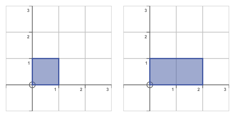
Example:

A =

[2 0]
[0 3]

Vector:

v = (1,2)

Result:

T(v) = (2,6)

This transformation stretches vectors differently along axes.


5. Geometric Interpretation

Linear transformations can change vectors in different ways:

  • Scaling
  • Rotation
  • Reflection
  • Shearing

However, they preserve the origin and straight lines.

Important properties:

  • Lines remain lines
  • Parallel lines remain parallel
  • Origin stays fixed

6. Types of Linear Transformations


Scaling Transformation

Scaling changes the size of vectors.

Example:

T(x,y) = (2x,3y)

Matrix:

[2 0]
[0 3]

Vectors stretch differently in each direction.


Rotation Transformation

Rotation rotates vectors around the origin.

Matrix:

[ cosθ −sinθ ]
[ sinθ cosθ ]

Example:

Rotation by 90°.


Reflection Transformation

Reflection flips vectors across a line.

Reflection across x-axis:

[1 0]
[0 −1]

Reflection across y-axis:

[-1 0]
[0 1]


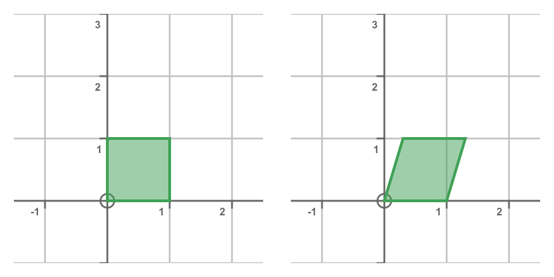
Shear Transformation

Shear transformation slants shapes.

Matrix:

[1 k]
[0 1]

Used in computer graphics.


7. Identity Transformation

The identity transformation leaves vectors unchanged.

Matrix:

[1 0]
[0 1]

T(v) = v


8. Zero Transformation

The zero transformation maps every vector to zero.

T(v) = 0

Matrix:

[0 0]
[0 0]


9. Composition of Transformations

Two transformations can be combined.

If:

T₁(v) = A v
T₂(v) = B v

Then composition:

T₂(T₁(v)) = BA v

This corresponds to matrix multiplication.


10. Kernel of a Linear Transformation

The kernel of a transformation is the set of vectors mapped to zero.

Kernel:

Ker(T) = {v | T(v) = 0}

It measures how much information is lost during transformation.


11. Image of a Transformation

The image (or range) is the set of all outputs.

Image:

Im(T) = {T(v)}

This represents all possible transformed vectors.


12. Rank and Nullity

Two important concepts are:

Rank = dimension of image
Nullity = dimension of kernel

These are related by:

Rank + Nullity = dimension of vector space

This is called the Rank–Nullity Theorem.


13. Invertible Transformations

A transformation is invertible if there exists another transformation that reverses it.

Example:

If

T(v) = Av

Then inverse:

T⁻¹(v) = A⁻¹v

Condition:

det(A) ≠ 0


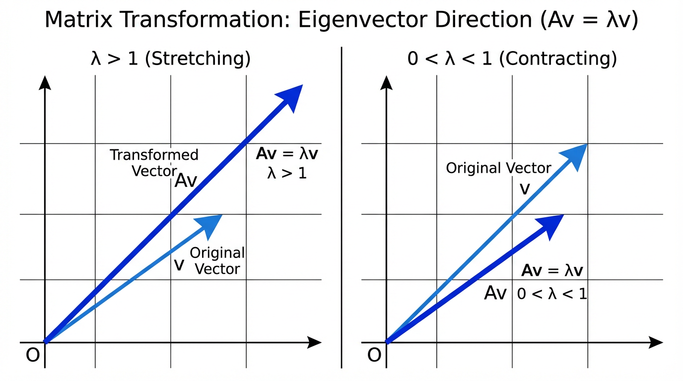
14. Eigenvalues and Linear Transformations

Eigenvalues describe how a transformation scales vectors.

Equation:

Av = λv

Where:

λ = eigenvalue
v = eigenvector

Eigenvectors remain in the same direction after transformation.


15. Diagonalization

Some transformations can be simplified using diagonal matrices.

A = PDP⁻¹

Where:

D contains eigenvalues.

This simplifies repeated transformations.


16. Linear Transformations in Geometry

In geometry, linear transformations manipulate shapes.

Examples:

  • Rotating objects
  • Scaling images
  • Reflecting shapes

Used extensively in computer graphics.


17. Linear Transformations in Physics

Physics uses transformations to describe physical systems.

Examples include:

  • rotation of coordinate systems
  • Lorentz transformations in relativity
  • quantum operators

These transformations help describe physical laws.


18. Applications in Computer Graphics

Linear transformations are essential in:

  • 3D modeling
  • video games
  • animation
  • virtual reality

Transformations allow objects to move, rotate, and scale.


19. Applications in Machine Learning

In machine learning, transformations are used to:

  • project data into new spaces
  • reduce dimensions
  • analyze features

Algorithms such as PCA rely on linear transformations.


20. Applications in Signal Processing

Signals can be represented as vectors.

Transformations help analyze signals using:

  • Fourier transforms
  • wavelet transforms

21. Linear Transformations in Robotics

Robots rely on transformations to calculate:

  • arm movements
  • rotations
  • coordinate conversions

Matrices help describe robot motion.


22. Importance of Linear Transformations

Linear transformations are powerful tools for understanding how vector spaces change under mathematical operations.

They allow mathematicians and scientists to model real-world processes efficiently.

They help simplify complex systems, analyze data, and perform geometric manipulations.


Conclusion

Linear transformations are fundamental operations in linear algebra that describe how vectors move or change within vector spaces. By preserving vector addition and scalar multiplication, these transformations maintain the underlying structure of vector spaces while allowing changes such as scaling, rotation, reflection, and shear.

Representing linear transformations using matrices makes calculations efficient and allows them to be applied to complex systems. Linear transformations form the foundation for many important mathematical concepts including eigenvalues, eigenvectors, and matrix diagonalization.

Their applications extend across many fields such as computer graphics, physics, engineering, robotics, machine learning, and signal processing. In modern technology, linear transformations are essential tools for manipulating data, modeling systems, and solving scientific problems.

Understanding linear transformations is therefore crucial for anyone studying advanced mathematics, data science, engineering, or computer science.


Tags

Eigenvalues and Eigenvectors

Image
Image
Image
Image

1. Introduction to Eigenvalues and Eigenvectors

Eigenvalues and eigenvectors are fundamental concepts in linear algebra and play a crucial role in many areas of mathematics, physics, engineering, and computer science. They help describe how linear transformations affect vectors in space.

When a matrix transforms a vector, the resulting vector may change in direction and magnitude. However, there are special vectors that only change in magnitude but not in direction when a transformation is applied. These vectors are called eigenvectors, and the factors by which they are scaled are called eigenvalues.

The word eigen comes from German, meaning “own” or “characteristic.” Therefore, eigenvalues and eigenvectors represent the characteristic properties of a matrix transformation.

In many scientific fields, eigenvalues and eigenvectors help analyze systems, identify patterns in data, and simplify complex mathematical problems. They are widely used in areas such as:

  • Quantum mechanics
  • Machine learning
  • Computer graphics
  • Structural engineering
  • Data analysis
  • Control systems
  • Image processing

Understanding eigenvalues and eigenvectors allows mathematicians and scientists to study the behavior of complex systems more effectively.


2. Linear Transformations and Matrices

Before understanding eigenvalues and eigenvectors, it is important to understand linear transformations.

A linear transformation is a mathematical operation that transforms vectors from one vector space to another while preserving the operations of addition and scalar multiplication.

In linear algebra, linear transformations are often represented using matrices.

For example, if matrix A acts on vector x, the transformation is written as:

Ax

Where:

A = transformation matrix
x = vector

This multiplication produces a new vector.

Most vectors change both direction and magnitude after transformation.

However, some special vectors only change magnitude while keeping the same direction.

These vectors are eigenvectors.


3. Definition of Eigenvalues and Eigenvectors

An eigenvector of a matrix is a vector that remains in the same direction after the matrix transformation.

An eigenvalue is the scalar value that represents how much the eigenvector is stretched or compressed.

Mathematically:

A v = λ v

Where:

A = square matrix
v = eigenvector
λ = eigenvalue

This equation means that multiplying matrix A by vector v gives the same vector scaled by λ.

If:

λ > 1 → vector stretches
0 < λ < 1 → vector shrinks
λ < 0 → vector reverses direction
λ = 0 → vector collapses to zero


4. Understanding the Concept Geometrically

Eigenvectors represent directions that remain unchanged during transformation.

When a transformation matrix acts on space:

  • Most vectors rotate or change direction
  • Eigenvectors only scale in magnitude

Imagine stretching a rubber sheet.

Some directions stretch directly without rotating.

These directions represent eigenvectors.

The stretching factor is the eigenvalue.


5. Finding Eigenvalues

To calculate eigenvalues of a matrix, we start from the equation:

A v = λ v

Rewrite it as:

A v − λ v = 0

Factor out v:

(A − λI)v = 0

Where:

I = identity matrix

For non-zero solutions:

det(A − λI) = 0

This equation is called the characteristic equation.

Solving it gives eigenvalues.


6. Example of Eigenvalue Calculation

Consider matrix:

A =

[2 1]
[1 2]

Step 1: Compute A − λI

A − λI =

[2−λ 1]
[1 2−λ]

Step 2: Find determinant

|2−λ 1|
|1 2−λ|

= (2−λ)(2−λ) − (1×1)

= (2−λ)² − 1

Expand:

= λ² − 4λ + 3

Step 3: Solve

λ² − 4λ + 3 = 0

(λ − 1)(λ − 3) = 0

Eigenvalues:

λ₁ = 1
λ₂ = 3


7. Finding Eigenvectors

Once eigenvalues are found, eigenvectors can be calculated.

Use equation:

(A − λI)v = 0

Example:

For eigenvalue λ = 3

A − 3I =

[-1 1]
[1 -1]

Solve system:

  • x + y = 0

y = x

Eigenvector:

[1
1]


8. Eigenvalues of Special Matrices

Certain matrices have simple eigenvalues.

Diagonal Matrix

Eigenvalues are diagonal elements.

Example:

[3 0 0]
[0 5 0]
[0 0 7]

Eigenvalues:

3, 5, 7


Identity Matrix

All eigenvalues = 1


Zero Matrix

All eigenvalues = 0


Triangular Matrix

Eigenvalues are diagonal elements.


9. Properties of Eigenvalues and Eigenvectors

Property 1

Sum of eigenvalues equals trace of matrix.

Trace = sum of diagonal elements.


Property 2

Product of eigenvalues equals determinant.


Property 3

Eigenvectors corresponding to different eigenvalues are linearly independent.


Property 4

Scaling a matrix scales eigenvalues.

If matrix multiplied by k:

Eigenvalues multiply by k.


Property 5

Eigenvalues of transpose matrix are the same.


10. Characteristic Polynomial

The equation:

det(A − λI) = 0

produces a polynomial called the characteristic polynomial.

Example:

λ² − 4λ + 3

Roots of this polynomial are eigenvalues.


11. Diagonalization of Matrices

Some matrices can be expressed in diagonal form.

A = PDP⁻¹

Where:

D = diagonal matrix of eigenvalues
P = matrix of eigenvectors

Diagonalization simplifies calculations.


12. Applications in Physics

Eigenvalues are widely used in physics.

Quantum Mechanics

Energy levels of atoms are eigenvalues of operators.

Example:

Schrödinger equation


Vibrations and Oscillations

Eigenvalues determine natural frequencies of structures.

Used in:

  • bridges
  • buildings
  • mechanical systems

13. Applications in Engineering

Eigenvalues help analyze:

  • stability of systems
  • mechanical vibrations
  • electrical circuits

In control systems, eigenvalues determine whether a system is stable.


14. Applications in Machine Learning

Eigenvalues and eigenvectors are used in:

Principal Component Analysis (PCA)

PCA reduces dimensionality of data.

Eigenvectors determine principal directions.

Eigenvalues measure importance of each component.


Face Recognition

Eigenfaces technique uses eigenvectors to represent facial images.


15. Applications in Computer Graphics

Eigenvalues help in:

  • geometric transformations
  • animation
  • image compression

Used to manipulate objects in 3D space.


16. Applications in Network Analysis

Eigenvectors help analyze networks.

Example:

Google PageRank algorithm uses eigenvectors to rank web pages.


17. Eigenvalues in Differential Equations

Eigenvalues help solve systems of differential equations.

Example:

Population models
Electrical circuits
Heat transfer problems


18. Eigenvalue Decomposition

Eigenvalue decomposition expresses matrix as:

A = VΛV⁻¹

Where:

Λ = diagonal matrix of eigenvalues
V = eigenvector matrix

Used in many numerical algorithms.


19. Singular Value Decomposition

SVD is related to eigenvalues.

It is used in:

  • recommendation systems
  • image compression
  • natural language processing

20. Importance of Eigenvalues and Eigenvectors

Eigenvalues and eigenvectors help simplify complex systems.

They allow:

  • analysis of transformations
  • dimensionality reduction
  • stability analysis
  • vibration analysis
  • pattern recognition

They are one of the most powerful tools in linear algebra.


Conclusion

Eigenvalues and eigenvectors are central concepts in linear algebra that describe the fundamental behavior of matrix transformations. They identify special directions in space that remain unchanged during transformation while only being scaled by a factor known as the eigenvalue.

These concepts provide deep insights into the structure of matrices and are essential for solving complex mathematical problems. Eigenvalues and eigenvectors are widely used in physics, engineering, computer science, and data science, enabling applications such as vibration analysis, machine learning, image processing, and network analysis.

By understanding eigenvalues and eigenvectors, researchers and engineers can simplify complicated systems, analyze stability, and uncover patterns in data. Their importance continues to grow as modern technology increasingly relies on advanced mathematical methods.


Tags