Tag Archives: eigenvectors

Eigenvalues and Eigenvectors

Image
Image
Image
Image

1. Introduction to Eigenvalues and Eigenvectors

Eigenvalues and eigenvectors are fundamental concepts in linear algebra and play a crucial role in many areas of mathematics, physics, engineering, and computer science. They help describe how linear transformations affect vectors in space.

When a matrix transforms a vector, the resulting vector may change in direction and magnitude. However, there are special vectors that only change in magnitude but not in direction when a transformation is applied. These vectors are called eigenvectors, and the factors by which they are scaled are called eigenvalues.

The word eigen comes from German, meaning “own” or “characteristic.” Therefore, eigenvalues and eigenvectors represent the characteristic properties of a matrix transformation.

In many scientific fields, eigenvalues and eigenvectors help analyze systems, identify patterns in data, and simplify complex mathematical problems. They are widely used in areas such as:

  • Quantum mechanics
  • Machine learning
  • Computer graphics
  • Structural engineering
  • Data analysis
  • Control systems
  • Image processing

Understanding eigenvalues and eigenvectors allows mathematicians and scientists to study the behavior of complex systems more effectively.


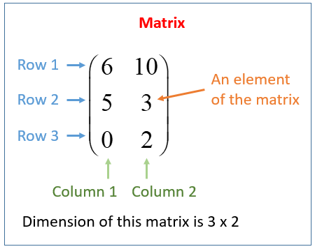
2. Linear Transformations and Matrices

Before understanding eigenvalues and eigenvectors, it is important to understand linear transformations.

A linear transformation is a mathematical operation that transforms vectors from one vector space to another while preserving the operations of addition and scalar multiplication.

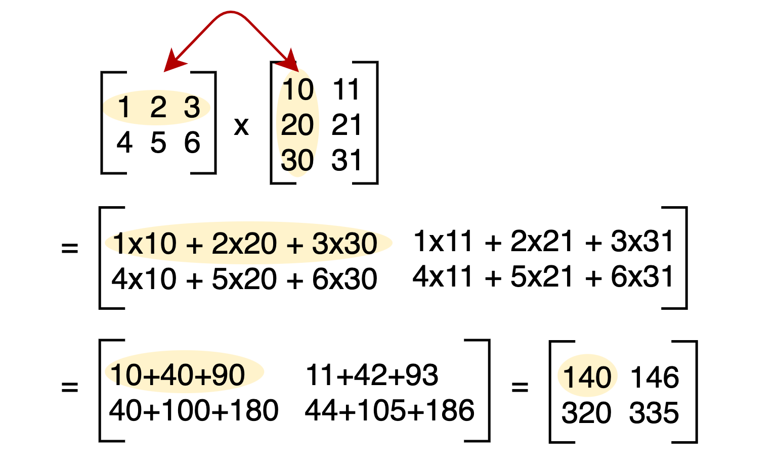
In linear algebra, linear transformations are often represented using matrices.

For example, if matrix A acts on vector x, the transformation is written as:

Ax

Where:

A = transformation matrix
x = vector

This multiplication produces a new vector.

Most vectors change both direction and magnitude after transformation.

However, some special vectors only change magnitude while keeping the same direction.

These vectors are eigenvectors.


3. Definition of Eigenvalues and Eigenvectors

An eigenvector of a matrix is a vector that remains in the same direction after the matrix transformation.

An eigenvalue is the scalar value that represents how much the eigenvector is stretched or compressed.

Mathematically:

A v = λ v

Where:

A = square matrix
v = eigenvector
λ = eigenvalue

This equation means that multiplying matrix A by vector v gives the same vector scaled by λ.
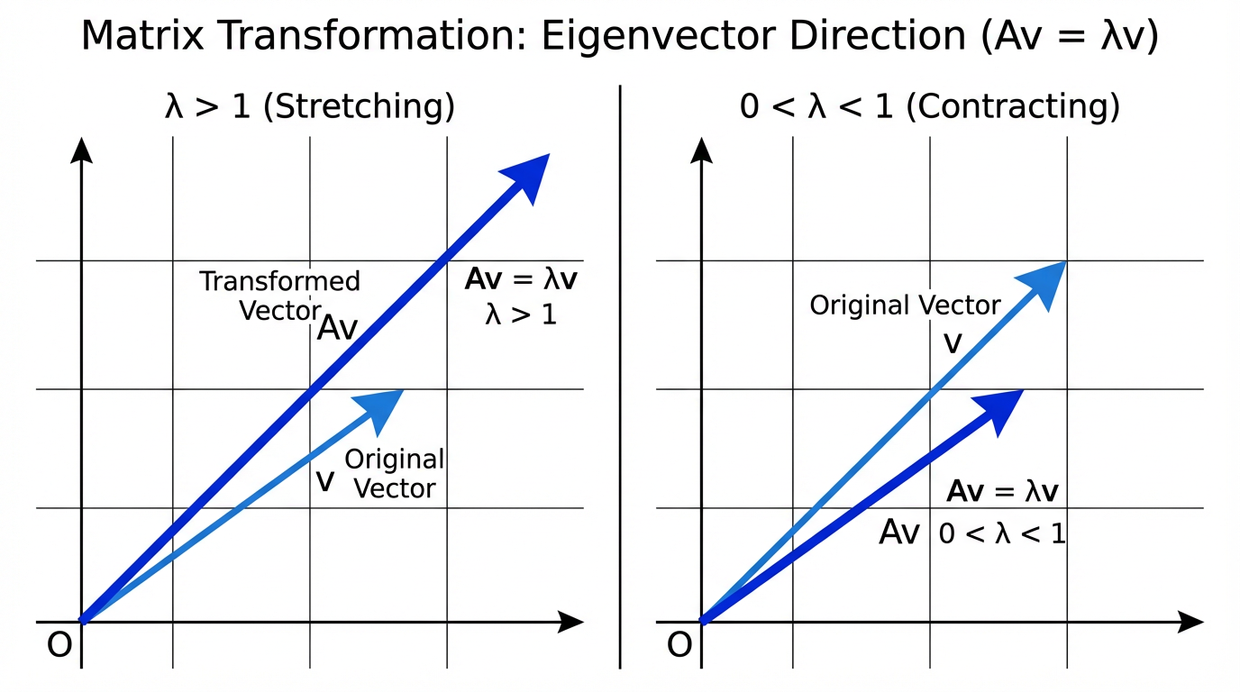
If:

λ > 1 → vector stretches
0 < λ < 1 → vector shrinks
λ < 0 → vector reverses direction
λ = 0 → vector collapses to zero


4. Understanding the Concept Geometrically

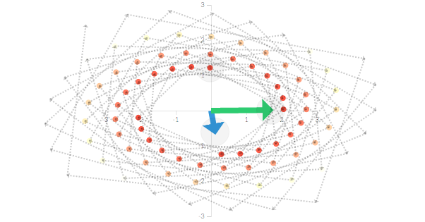
Eigenvectors represent directions that remain unchanged during transformation.

When a transformation matrix acts on space:

  • Most vectors rotate or change direction
  • Eigenvectors only scale in magnitude

Imagine stretching a rubber sheet.

Some directions stretch directly without rotating.

These directions represent eigenvectors.

The stretching factor is the eigenvalue.


5. Finding Eigenvalues

To calculate eigenvalues of a matrix, we start from the equation:

A v = λ v

Rewrite it as:

A v − λ v = 0

Factor out v:

(A − λI)v = 0

Where:

I = identity matrix

For non-zero solutions:

det(A − λI) = 0

This equation is called the characteristic equation.

Solving it gives eigenvalues.


6. Example of Eigenvalue Calculation

Consider matrix:

A =

[2 1]
[1 2]

Step 1: Compute A − λI

A − λI =

[2−λ 1]
[1 2−λ]

Step 2: Find determinant

|2−λ 1|
|1 2−λ|

= (2−λ)(2−λ) − (1×1)

= (2−λ)² − 1

Expand:

= λ² − 4λ + 3

Step 3: Solve

λ² − 4λ + 3 = 0

(λ − 1)(λ − 3) = 0

Eigenvalues:

λ₁ = 1
λ₂ = 3


7. Finding Eigenvectors

Once eigenvalues are found, eigenvectors can be calculated.

Use equation:

(A − λI)v = 0

Example:

For eigenvalue λ = 3

A − 3I =

[-1 1]
[1 -1]

Solve system:

  • x + y = 0

y = x

Eigenvector:

[1
1]


8. Eigenvalues of Special Matrices

Certain matrices have simple eigenvalues.

Diagonal Matrix

Eigenvalues are diagonal elements.

Example:

[3 0 0]
[0 5 0]
[0 0 7]

Eigenvalues:

3, 5, 7


Identity Matrix

All eigenvalues = 1


Zero Matrix

All eigenvalues = 0


Triangular Matrix

Eigenvalues are diagonal elements.


9. Properties of Eigenvalues and Eigenvectors

Property 1

Sum of eigenvalues equals trace of matrix.

Trace = sum of diagonal elements.


Property 2

Product of eigenvalues equals determinant.


Property 3

Eigenvectors corresponding to different eigenvalues are linearly independent.


Property 4

Scaling a matrix scales eigenvalues.

If matrix multiplied by k:

Eigenvalues multiply by k.


Property 5

Eigenvalues of transpose matrix are the same.


10. Characteristic Polynomial

The equation:

det(A − λI) = 0

produces a polynomial called the characteristic polynomial.

Example:

λ² − 4λ + 3

Roots of this polynomial are eigenvalues.


11. Diagonalization of Matrices

Some matrices can be expressed in diagonal form.

A = PDP⁻¹

Where:

D = diagonal matrix of eigenvalues
P = matrix of eigenvectors

Diagonalization simplifies calculations.


12. Applications in Physics

Eigenvalues are widely used in physics.

Quantum Mechanics

Energy levels of atoms are eigenvalues of operators.

Example:

Schrödinger equation


Vibrations and Oscillations

Eigenvalues determine natural frequencies of structures.

Used in:

  • bridges
  • buildings
  • mechanical systems

13. Applications in Engineering

Eigenvalues help analyze:

  • stability of systems
  • mechanical vibrations
  • electrical circuits

In control systems, eigenvalues determine whether a system is stable.


14. Applications in Machine Learning

Eigenvalues and eigenvectors are used in:

Principal Component Analysis (PCA)

PCA reduces dimensionality of data.

Eigenvectors determine principal directions.

Eigenvalues measure importance of each component.


Face Recognition

Eigenfaces technique uses eigenvectors to represent facial images.


15. Applications in Computer Graphics

Eigenvalues help in:

  • geometric transformations
  • animation
  • image compression

Used to manipulate objects in 3D space.


16. Applications in Network Analysis

Eigenvectors help analyze networks.

Example:

Google PageRank algorithm uses eigenvectors to rank web pages.


17. Eigenvalues in Differential Equations

Eigenvalues help solve systems of differential equations.

Example:

Population models
Electrical circuits
Heat transfer problems


18. Eigenvalue Decomposition

Eigenvalue decomposition expresses matrix as:

A = VΛV⁻¹

Where:

Λ = diagonal matrix of eigenvalues
V = eigenvector matrix

Used in many numerical algorithms.


19. Singular Value Decomposition

SVD is related to eigenvalues.

It is used in:

  • recommendation systems
  • image compression
  • natural language processing

20. Importance of Eigenvalues and Eigenvectors

Eigenvalues and eigenvectors help simplify complex systems.

They allow:

  • analysis of transformations
  • dimensionality reduction
  • stability analysis
  • vibration analysis
  • pattern recognition

They are one of the most powerful tools in linear algebra.


Conclusion

Eigenvalues and eigenvectors are central concepts in linear algebra that describe the fundamental behavior of matrix transformations. They identify special directions in space that remain unchanged during transformation while only being scaled by a factor known as the eigenvalue.

These concepts provide deep insights into the structure of matrices and are essential for solving complex mathematical problems. Eigenvalues and eigenvectors are widely used in physics, engineering, computer science, and data science, enabling applications such as vibration analysis, machine learning, image processing, and network analysis.

By understanding eigenvalues and eigenvectors, researchers and engineers can simplify complicated systems, analyze stability, and uncover patterns in data. Their importance continues to grow as modern technology increasingly relies on advanced mathematical methods.


Tags

Matrices

Image
Image
Image
Image

1. Introduction to Matrices

A matrix is a rectangular arrangement of numbers, symbols, or expressions organized in rows and columns. Matrices are one of the most important structures in mathematics and play a crucial role in algebra, engineering, physics, statistics, computer science, economics, and data science.

Matrices are particularly useful when dealing with large sets of numbers, solving systems of linear equations, performing transformations in geometry, and modeling real-world problems.

The plural of matrix is matrices.

Matrices were first introduced in the 19th century by mathematicians such as Arthur Cayley, who developed matrix algebra. Since then, matrices have become a fundamental component of linear algebra, which is widely used in scientific and technological applications.

For example, consider a simple table representing students’ marks:

MathScienceEnglish
857890
888291

This table can be represented as a matrix:

A =
[ 85 78 90 ]
[ 88 82 91 ]

Each number in a matrix is called an element or entry.


2. Structure of a Matrix

A matrix is defined by:

  • Rows
  • Columns

If a matrix has m rows and n columns, it is called an m × n matrix.

Example:

A =
[ 1 2 3 ]
[ 4 5 6 ]

This matrix has:

Rows = 2
Columns = 3

So it is called a 2 × 3 matrix.


General Form of a Matrix

A matrix is usually written as:

A = [aᵢⱼ]

Where:

  • i represents row number
  • j represents column number

Example:

A =
[ a11 a12 a13 ]
[ a21 a22 a23 ]

Here:

a21 means element in 2nd row and 1st column.


3. Representation of Matrices

Matrices are represented using capital letters.

Examples:

A, B, C, M, X

Example matrix:

A =
[ 2 5 ]
[ 3 7 ]

The elements are:

a11 = 2
a12 = 5
a21 = 3
a22 = 7


4. Order of a Matrix

The order of a matrix describes its size.

Order = rows × columns

Examples:

MatrixOrder
[1 2]1 × 2
[3 4; 5 6]2 × 2
[1 2 3; 4 5 6; 7 8 9]3 × 3

5. Types of Matrices

Matrices can be classified into several types based on their structure.


Row Matrix

A matrix with only one row.

Example:

A = [ 2 4 6 8 ]

Order:

1 × 4


Column Matrix

A matrix with only one column.

Example:

A =
[3]
[5]
[7]

Order:

3 × 1


Rectangular Matrix

If rows ≠ columns.

Example:

2 × 3 matrix

A =
[1 2 3]
[4 5 6]


Square Matrix

A matrix with equal rows and columns.

Example:

A =
[1 2]
[3 4]

Order:

2 × 2

Square matrices are very important because many operations like determinants and inverses are defined for them.


Zero Matrix

A matrix whose elements are all zero.

Example:

A =
[0 0]
[0 0]


Diagonal Matrix

A square matrix where all elements except the diagonal are zero.

Example:

A =
[5 0 0]
[0 3 0]
[0 0 7]


Identity Matrix

A square matrix where diagonal elements are 1 and others are 0.

Example:

I =
[1 0 0]
[0 1 0]
[0 0 1]

Identity matrix behaves like number 1 in multiplication.


Scalar Matrix

A diagonal matrix with equal diagonal elements.

Example:

A =
[4 0 0]
[0 4 0]
[0 0 4]


Upper Triangular Matrix

Elements below the diagonal are zero.

Example:

A =
[2 4 6]
[0 5 7]
[0 0 9]


Lower Triangular Matrix

Elements above the diagonal are zero.

Example:

A =
[3 0 0]
[5 6 0]
[7 8 9]


6. Equality of Matrices

Two matrices are equal if:

  1. Their orders are equal
  2. Corresponding elements are equal

Example:

A =
[1 2]
[3 4]

B =
[1 2]
[3 4]

Therefore:

A = B


7. Addition of Matrices

Matrices can be added if they have the same order.

Example:

A =
[1 2]
[3 4]

B =
[5 6]
[7 8]

A + B =

[1+5 2+6]
[3+7 4+8]

Result:

[6 8]
[10 12]


Properties of Matrix Addition

  1. Commutative Property

A + B = B + A

  1. Associative Property

(A + B) + C = A + (B + C)

  1. Additive Identity

A + 0 = A

  1. Additive Inverse

A + (-A) = 0


8. Subtraction of Matrices

Matrix subtraction is defined as:

A − B = A + (−B)

Example:

A =
[8 6]
[4 2]

B =
[3 1]
[5 2]

A − B =

[5 5]
[-1 0]


9. Scalar Multiplication

Multiplying a matrix by a number.

Example:

A =
[2 4]
[6 8]

3A =

[6 12]
[18 24]


10. Matrix Multiplication

Matrix multiplication is different from ordinary multiplication.

Condition:

Columns of first matrix = rows of second matrix

If

A = m × n
B = n × p

Then:

AB = m × p


Example:

A =
[1 2]
[3 4]

B =
[5 6]
[7 8]

AB =

[1×5 + 2×7 1×6 + 2×8]
[3×5 + 4×7 3×6 + 4×8]

Result:

[19 22]
[43 50]


Properties of Matrix Multiplication

  1. Not commutative

AB ≠ BA

  1. Associative

(A B)C = A(B C)

  1. Distributive

A(B + C) = AB + AC


11. Transpose of a Matrix

The transpose of a matrix is obtained by interchanging rows and columns.

If A is matrix:

Aᵀ is transpose.

Example:

A =
[1 2 3]
[4 5 6]

Aᵀ =

[1 4]
[2 5]
[3 6]


12. Determinant of a Matrix

Determinants are defined only for square matrices.

For a 2×2 matrix

A =
[ a b ]
[ c d ]

Determinant:

|A| = ad − bc

Example:

| 2 3 |
| 4 5 |

= (2×5) − (3×4)
= 10 − 12
= −2


13. Inverse of a Matrix

A matrix inverse is similar to reciprocal.

If:

A⁻¹ exists then

A × A⁻¹ = I

Where I is identity matrix.

For 2×2 matrix:

A =
[ a b ]
[ c d ]

Inverse:

1/(ad − bc)

[ d −b ]
[ −c a ]


14. Rank of a Matrix

The rank of a matrix is the maximum number of independent rows or columns.

Rank tells:

  • how many independent equations exist
  • whether system has solution

15. Elementary Operations on Matrices

Three basic operations:

  1. Row swapping
  2. Row multiplication
  3. Row addition

Used in solving equations.


16. Systems of Linear Equations Using Matrices

Example system:

2x + y = 5
x + 3y = 7

Matrix form:

AX = B

A = coefficient matrix
X = variable matrix
B = constant matrix

Using inverse:

X = A⁻¹B


17. Applications of Matrices

Matrices are used in many fields.


Computer Graphics

Matrices perform transformations:

  • Rotation
  • Scaling
  • Translation

Used in video games and animation.


Physics

Matrices describe:

  • Quantum mechanics
  • Electromagnetism
  • Mechanics

Engineering

Used in:

  • Structural analysis
  • Electrical circuits
  • Robotics

Economics

Matrices help analyze:

  • Input-output models
  • Economic forecasting

Statistics

Matrices represent datasets and perform calculations like:

  • covariance
  • regression
  • machine learning algorithms

Cryptography

Matrices are used in encryption methods like the Hill cipher.


Artificial Intelligence

Matrices represent:

  • neural networks
  • machine learning data
  • deep learning models

18. Matrices in Computer Science

Matrices play a major role in:

  • Image processing
  • Data compression
  • Graph theory
  • Machine learning

Example:

Images are stored as pixel matrices.


19. Eigenvalues and Eigenvectors

For a matrix A:

Av = λv

Where:

λ = eigenvalue
v = eigenvector

These concepts are used in:

  • vibration analysis
  • facial recognition
  • Google PageRank

20. Importance of Matrices

Matrices simplify complex mathematical problems.

They help in:

  • solving simultaneous equations
  • modeling systems
  • handling large datasets
  • performing transformations

Matrices are essential tools in modern science and technology.


Conclusion

Matrices are powerful mathematical tools that organize numbers into structured arrays. They play a central role in linear algebra and are widely used in mathematics, engineering, physics, computer science, economics, and artificial intelligence. By representing complex data and relationships in a compact form, matrices make it easier to perform calculations, solve equations, and analyze systems.

Matrix operations such as addition, multiplication, transpose, determinants, and inverses allow mathematicians and scientists to model real-world problems effectively. Applications of matrices extend to computer graphics, machine learning, quantum physics, robotics, and cryptography.

Understanding matrices provides a foundation for advanced mathematical concepts and modern technological developments.


Tags