


1. Introduction to Electron Configuration
Electron configuration is the arrangement of electrons in the orbitals of an atom or molecule. It describes how electrons occupy different energy levels and subshells around the nucleus. Understanding electron configuration is fundamental to chemistry because it explains the chemical behavior of elements, including their bonding properties, reactivity, and position in the periodic table.
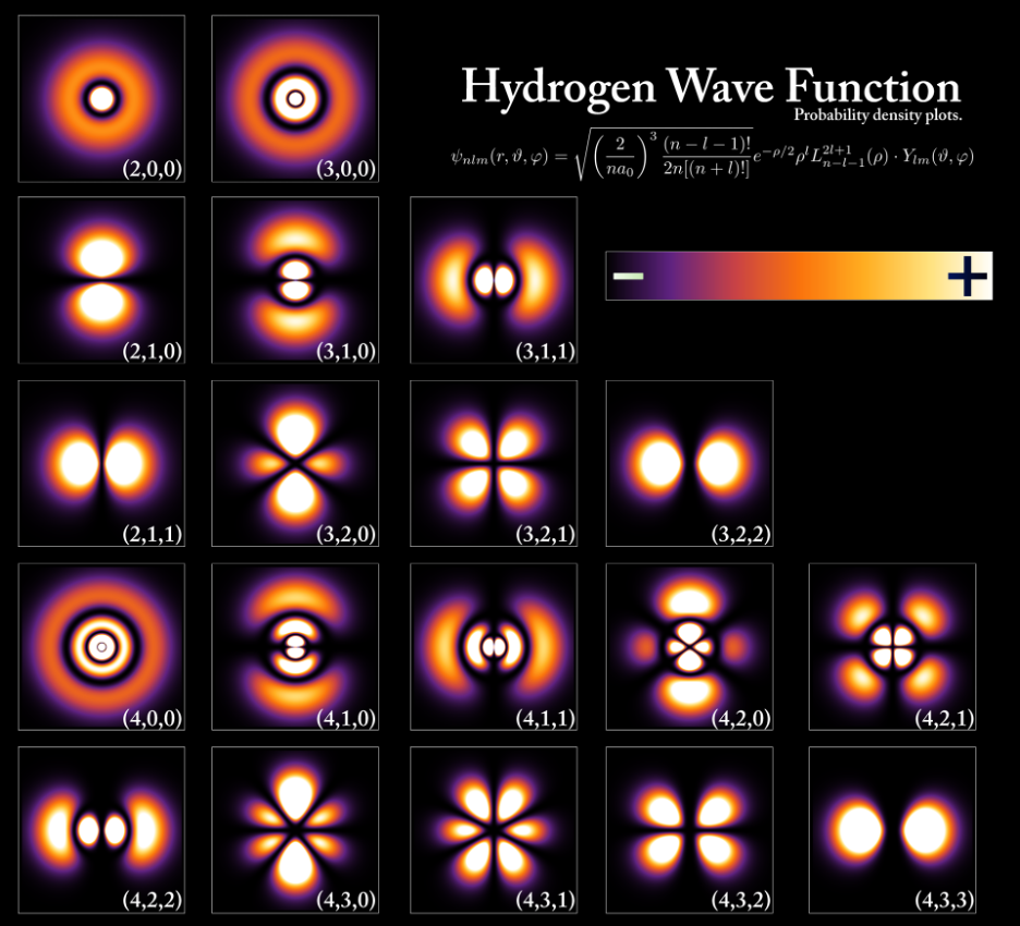
Electrons occupy regions around the nucleus known as atomic orbitals. These orbitals represent probability distributions where electrons are most likely to be found. The distribution of electrons among these orbitals follows specific rules derived from quantum mechanics.
Electron configuration helps explain many important chemical phenomena, including:
- Periodic trends in the periodic table
- Chemical bonding and molecular structure
- Ion formation
- Magnetic properties of substances
- Spectroscopic behavior of atoms
The concept of electron configuration emerged from the development of quantum mechanics in the early twentieth century. Scientists such as Niels Bohr, Erwin Schrödinger, and Wolfgang Pauli contributed to the understanding of electron behavior in atoms.
Each element has a unique electron configuration determined by the number of electrons in its atoms. For neutral atoms, the number of electrons equals the number of protons in the nucleus.
Electron configuration provides insight into the stability of atoms and their tendency to gain, lose, or share electrons during chemical reactions.
2. Energy Levels and Atomic Orbitals

Electrons in atoms occupy specific energy levels known as shells. Each shell contains one or more subshells, and each subshell contains orbitals.
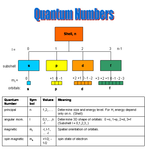
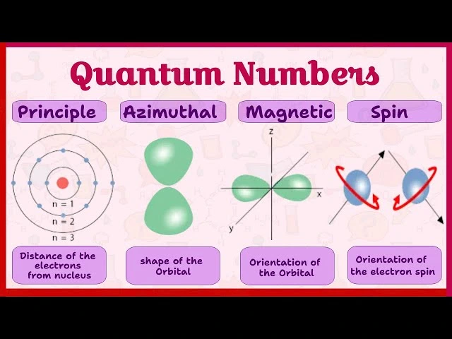
Principal Energy Levels
The principal energy level is represented by the principal quantum number (n).
Possible values of n are:
1, 2, 3, 4, …
As the value of n increases:
- The energy of electrons increases.
- The average distance from the nucleus increases.
- The orbitals become larger.
Each energy level can hold a maximum number of electrons given by the formula:
Maximum electrons = 2n²
Examples:
n = 1 → 2 electrons
n = 2 → 8 electrons
n = 3 → 18 electrons
n = 4 → 32 electrons
Subshells
Each principal energy level contains subshells defined by the azimuthal quantum number (l).
Subshell types include:
- s subshell
- p subshell
- d subshell
- f subshell
Each subshell contains a specific number of orbitals.
Orbitals
Orbitals are regions in space where electrons are most likely to be found.
Each orbital can hold a maximum of two electrons with opposite spins.
Number of orbitals in each subshell:
s subshell → 1 orbital → 2 electrons
p subshell → 3 orbitals → 6 electrons
d subshell → 5 orbitals → 10 electrons
f subshell → 7 orbitals → 14 electrons
3. Principles Governing Electron Configuration


Electron configuration follows three important principles.
Aufbau Principle
The Aufbau principle states that electrons fill orbitals in order of increasing energy.
Lower-energy orbitals are filled before higher-energy orbitals.
This principle determines the sequence in which orbitals are filled.
Orbital filling order generally follows:
1s → 2s → 2p → 3s → 3p → 4s → 3d → 4p → 5s → 4d → 5p → 6s → 4f → 5d → 6p → 7s
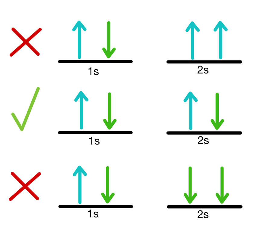
Pauli Exclusion Principle
The Pauli Exclusion Principle states that:
No two electrons in an atom can have the same set of four quantum numbers.
Because of this rule:
- Each orbital holds at most two electrons.
- These electrons must have opposite spins.
Hund’s Rule
Hund’s rule states that electrons occupy orbitals singly before pairing.
When multiple orbitals of the same energy are available, electrons fill them one at a time with parallel spins.
This arrangement minimizes electron repulsion and increases stability.
4. Writing Electron Configurations


Electron configurations are written using a notation that indicates:
- Energy level (n)
- Subshell (s, p, d, f)
- Number of electrons in the subshell
Example:
Hydrogen:
1s¹
Helium:
1s²
Lithium:
1s² 2s¹
Carbon:
1s² 2s² 2p²
Oxygen:
1s² 2s² 2p⁴
This notation shows how electrons are distributed across orbitals.
Orbital Diagrams
Orbital diagrams represent orbitals as boxes and electrons as arrows.
Example for carbon:
1s ↑↓
2s ↑↓
2p ↑ ↑
The arrows represent electron spin.
5. Noble Gas Configuration


To simplify electron configurations for large atoms, scientists use noble gas shorthand notation.
In this method:
- The electron configuration of the nearest noble gas is used as a core.
- Remaining electrons are written after the noble gas symbol.
Example:
Sodium:
Full configuration:
1s² 2s² 2p⁶ 3s¹
Shorthand:
[Ne] 3s¹
Iron:
[Ar] 4s² 3d⁶
This notation makes electron configurations easier to write and understand.
6. Electron Configuration and the Periodic Table


The structure of the periodic table is directly related to electron configuration.
Elements are arranged according to the filling of orbitals.
s-block
Includes Groups 1 and 2.
Electrons are added to s orbitals.
p-block
Includes Groups 13–18.
Electrons fill p orbitals.
d-block
Contains transition metals.
Electrons fill d orbitals.
f-block
Includes lanthanides and actinides.
Electrons fill f orbitals.
This arrangement explains periodic trends such as atomic radius and ionization energy.
7. Exceptions to Electron Configuration
Although the Aufbau principle generally predicts electron configurations accurately, there are exceptions.
These occur when half-filled or fully filled subshells provide extra stability.
Examples include:
Chromium:
Expected:
[Ar] 4s² 3d⁴
Actual:
[Ar] 4s¹ 3d⁵
Copper:
Expected:
[Ar] 4s² 3d⁹
Actual:
[Ar] 4s¹ 3d¹⁰
These exceptions occur because half-filled and fully filled d subshells are more stable.
8. Electron Configuration of Ions
Atoms can gain or lose electrons to form ions.
Cations
Positive ions form when atoms lose electrons.
Example:
Sodium:
Na → Na⁺ + e⁻
Electron configuration:
Na: [Ne] 3s¹
Na⁺: [Ne]
Anions
Negative ions form when atoms gain electrons.
Example:
Chlorine:
Cl + e⁻ → Cl⁻
Electron configuration:
Cl: [Ne] 3s² 3p⁵
Cl⁻: [Ne] 3s² 3p⁶
Ion formation often results in noble gas configurations, which are highly stable.
9. Electron Configuration and Chemical Bonding
Electron configuration determines how atoms interact during chemical reactions.
Atoms tend to achieve stable electron arrangements similar to noble gases.
This occurs through:
- Electron transfer (ionic bonding)
- Electron sharing (covalent bonding)
- Electron pooling (metallic bonding)
Valence electrons—the electrons in the outermost shell—play the most important role in bonding.
10. Magnetic Properties and Electron Configuration
Electron configuration influences the magnetic behavior of substances.
Diamagnetic Substances
Atoms with all electrons paired are diamagnetic.
They are weakly repelled by magnetic fields.
Paramagnetic Substances
Atoms with unpaired electrons are paramagnetic.
They are attracted to magnetic fields.
Transition metals often show paramagnetism due to unpaired d electrons.
11. Applications of Electron Configuration
Electron configuration has many applications in science and technology.
Chemical Reactivity
It helps predict how elements react and form compounds.
Spectroscopy
Electron transitions between orbitals produce characteristic spectral lines.
Materials Science
Understanding electron arrangements helps design semiconductors and superconductors.
Quantum Chemistry
Electron configurations form the basis for theoretical calculations of molecular behavior.
Nanotechnology
Manipulating electron behavior allows the development of advanced nanoscale materials.
12. Conclusion
Electron configuration is a fundamental concept in chemistry that describes the arrangement of electrons within atoms. It provides deep insight into atomic structure, chemical bonding, and the periodic organization of elements.
By following the principles of the Aufbau rule, Pauli exclusion principle, and Hund’s rule, electrons fill atomic orbitals in predictable patterns. These patterns explain the stability, reactivity, and physical properties of elements.
Electron configuration also plays a crucial role in modern scientific fields such as spectroscopy, materials science, nanotechnology, and quantum chemistry.
Understanding electron configuration allows scientists to interpret atomic behavior and design new technologies based on the manipulation of electrons.