Author Archives: AI Education

Circular Motion

Image
Image
Image
Image

Introduction

Circular motion is a type of motion in which an object moves along a circular path around a fixed point or axis. It is one of the most important types of motion studied in classical mechanics. Unlike motion in a straight line, circular motion involves continuous change in direction, even if the speed of the object remains constant.

Many natural and artificial systems exhibit circular motion. Examples include the motion of planets around the Sun, electrons moving around atomic nuclei, cars moving around circular tracks, rotating wheels, satellites orbiting Earth, and amusement park rides such as merry-go-rounds.

Circular motion is significant because it introduces the concept of centripetal acceleration and centripetal force, which are necessary to keep an object moving along a curved path. Without these forces, objects would move in straight lines according to Newton’s first law of motion.

In circular motion, several important quantities are studied, including angular displacement, angular velocity, angular acceleration, centripetal force, and tangential velocity. Understanding these quantities allows physicists and engineers to analyze rotating systems and orbital motion.

Circular motion plays a crucial role in many fields such as physics, astronomy, engineering, robotics, and transportation systems.


Basic Concepts of Circular Motion

Definition of Circular Motion

Circular motion is defined as the motion of an object along the circumference of a circle or a circular path.

The center of the circle is called the axis of rotation, and the distance between the center and the object is called the radius of the circular path.

In circular motion, even if the speed remains constant, the direction of motion changes continuously. This change in direction results in acceleration.


Examples of Circular Motion

Examples of circular motion appear frequently in everyday life and nature.

Examples include:

  • A stone tied to a string and rotated in a circle
  • Blades of a rotating fan
  • Motion of satellites around Earth
  • Wheels of a moving vehicle
  • Motion of planets around the Sun
  • Rotating turbines in power plants

All of these systems involve objects moving along circular paths.


Types of Circular Motion

Circular motion can be classified into two main types.


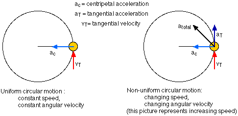
Uniform Circular Motion

Uniform circular motion occurs when an object moves along a circular path with constant speed.

Although the speed remains constant, the direction of velocity changes continuously. Therefore, acceleration is present.

Examples include:

  • Earth orbiting the Sun
  • A car moving at constant speed around a circular track
  • A rotating fan blade

Non-Uniform Circular Motion

Non-uniform circular motion occurs when the speed of the object changes while moving in a circular path.

In this case, acceleration occurs due to:

  • Change in speed
  • Change in direction

Examples include:

  • A car accelerating around a circular track
  • A rotating disk that speeds up or slows down

Angular Quantities in Circular Motion

In circular motion, angular quantities are often used to describe rotation.


Angular Displacement

Angular displacement represents the angle through which an object rotates.

It is measured in radians.

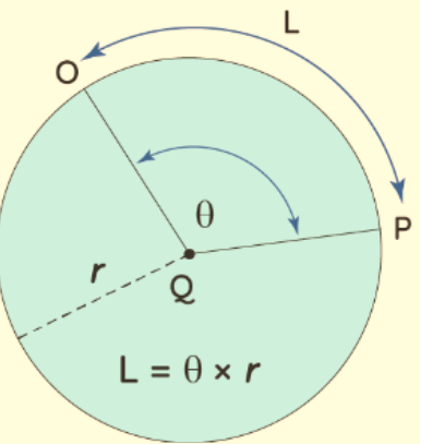
[
\theta = \frac{s}{r}
]

Where:

(s) = arc length
(r) = radius of circle


Angular Velocity

Angular velocity describes the rate of change of angular displacement.

[
\omega = \frac{\theta}{t}
]

Where:

(\omega) = angular velocity
(\theta) = angular displacement
(t) = time

Unit of angular velocity:

[
rad/s
]


Angular Acceleration

Angular acceleration represents the rate of change of angular velocity.

[
\alpha = \frac{d\omega}{dt}
]

Unit:

[
rad/s^2
]


Relationship Between Linear and Angular Motion
Image
Image
Image
Image

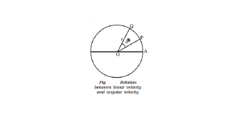
Linear and angular quantities are related.

Linear Velocity

The linear velocity of an object moving in a circle is given by:

[
v = r\omega
]

Where:

(v) = linear velocity
(r) = radius
(\omega) = angular velocity

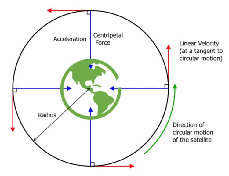
Linear velocity acts tangentially to the circular path.


Centripetal Acceleration

Even when an object moves at constant speed in a circle, it experiences acceleration because its direction changes continuously.

This acceleration is called centripetal acceleration.

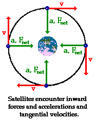
The centripetal acceleration always points toward the center of the circle.

[
a_c = \frac{v^2}{r}
]

Where:

(v) = velocity
(r) = radius

Another expression is:

[
a_c = r\omega^2
]


Centripetal Force

Image
Image
Image
Image

Centripetal force is the force required to keep an object moving in a circular path.

Without centripetal force, the object would move in a straight line according to Newton’s first law.

The formula for centripetal force is:

[
F_c = \frac{mv^2}{r}
]

Where:

(m) = mass
(v) = velocity
(r) = radius

Alternatively:

[
F_c = mr\omega^2
]


Sources of Centripetal Force

Different forces can provide centripetal force in different situations.

Examples include:

Gravitational force → planetary motion

Tension force → stone tied to string

Frictional force → car moving on curved road

Normal force → roller coaster motion


Centrifugal Force

Centrifugal force is an apparent force observed in a rotating reference frame.

It appears to push objects away from the center of the circular path.

Examples include:

Passengers pushed outward in a turning car.

Clothes sticking to the walls of a spinning washing machine.

Centrifugal force is considered a pseudo force because it appears due to the rotating frame of reference.


Period and Frequency

Two important quantities related to circular motion are period and frequency.


Period

The period is the time required for one complete revolution.

[
T = \frac{1}{f}
]

Unit: seconds


Frequency

Frequency is the number of revolutions per second.

[
f = \frac{1}{T}
]

Unit: Hertz (Hz)


Angular Velocity Relation

Angular velocity is related to period and frequency.

[
\omega = \frac{2\pi}{T}
]

or

[
\omega = 2\pi f
]


Applications of Circular Motion

Circular motion has many practical applications.

Planetary Motion

Planets revolve around the Sun due to gravitational centripetal force.

Satellites

Artificial satellites orbit Earth using gravitational force.

Transportation

Vehicles turning on curved roads experience circular motion.

Engineering

Rotating machinery such as turbines and engines use circular motion.

Sports

Hammer throw and discus events involve circular motion.

Amusement Parks

Rides such as roller coasters and merry-go-rounds use circular motion principles.


Banking of Roads

When vehicles move along curved roads, they require centripetal force.

To provide this force safely, roads are often banked.

Banking tilts the road surface so that the normal force helps provide centripetal force.

This reduces dependence on friction and prevents skidding.


Vertical Circular Motion

Vertical circular motion occurs when an object moves in a circular path in a vertical plane.

Examples include:

  • Roller coaster loops
  • Swinging bucket of water
  • Pendulum motion

In vertical circular motion, the speed changes due to gravity.

At the top of the circle, the object must have sufficient velocity to maintain the circular path.


Importance of Circular Motion

Circular motion is fundamental in physics because many natural phenomena involve rotational movement.

Important fields using circular motion include:

Astrophysics
Mechanical engineering
Electrical engineering
Robotics
Transportation engineering

Understanding circular motion allows scientists to design stable orbits, efficient engines, and safe transportation systems.


Summary

Circular motion is the motion of an object along a circular path around a central point. It involves constant change in direction, which leads to centripetal acceleration even when speed remains constant.

Key concepts in circular motion include angular displacement, angular velocity, centripetal force, and centripetal acceleration. These concepts help explain how objects remain in circular paths.

Circular motion is observed in many systems such as planetary orbits, rotating machines, vehicles on curved roads, and amusement park rides. By understanding circular motion, scientists and engineers can design technologies and explain many natural phenomena.

Circular motion remains one of the most important topics in mechanics and plays a vital role in understanding rotational dynamics and orbital mechanics.


Tags

Force and Friction

Image
Image
Image
Image

Introduction

In physics, the concept of force plays a fundamental role in understanding motion and interactions between objects. Every movement or change in motion occurs because of forces acting on objects. When a person pushes a door, pulls a rope, kicks a ball, or lifts a book, forces are involved.

Force is defined as a push or pull acting on an object that can change its state of motion, shape, or direction. It is one of the most important concepts in classical mechanics and forms the foundation of Newton’s laws of motion.

One particular type of force that plays a major role in everyday life is friction. Friction is the force that opposes motion between two surfaces that are in contact with each other. Without friction, many everyday activities such as walking, driving vehicles, or writing with a pencil would not be possible.

Understanding force and friction allows scientists and engineers to design machines, vehicles, and structures that function efficiently. These concepts are also essential in fields such as mechanical engineering, aerospace engineering, robotics, and biomechanics.


Force

Definition of Force

Force is defined as an interaction that causes an object to accelerate, decelerate, change direction, or change shape.

Mathematically, force is related to acceleration through Newton’s second law:

[
F = ma
]

Where:

  • (F) = force
  • (m) = mass
  • (a) = acceleration

Force is a vector quantity, meaning it has both magnitude and direction.


Unit of Force

The SI unit of force is the Newton (N).

One Newton is defined as the force required to accelerate a mass of 1 kilogram by 1 meter per second squared.

[
1N = 1,kg \cdot m/s^2
]

Other units sometimes used include:

Dyne (CGS unit)

[
1N = 10^5 , dyne
]


Characteristics of Force

Force has several important characteristics:

  1. Force has magnitude.
  2. Force has direction.
  3. Force can change the speed of an object.
  4. Force can change the direction of motion.
  5. Force can change the shape of an object.

For example:

  • Compressing a spring changes its shape.
  • Pushing a car causes it to move.
  • Applying brakes slows a vehicle.

Types of Forces

Forces in physics are categorized into different types based on their origin and how they act.


Contact Forces

Contact forces act only when two objects physically touch each other.

Examples include:

Frictional Force

Force opposing motion between surfaces.

Normal Force

Force exerted by a surface supporting an object.

Tension Force

Force transmitted through a string or rope.

Applied Force

Force exerted by a person or object.

Air Resistance

Force opposing motion through air.


Non-Contact Forces

Non-contact forces act without physical contact between objects.

Examples include:

Gravitational Force

Force of attraction between masses.

Magnetic Force

Force between magnetic objects.

Electrostatic Force

Force between electric charges.


Representation of Forces

Forces are represented using vectors.

A force vector shows:

  • Magnitude (length of arrow)
  • Direction (orientation of arrow)

For example:

A force of 10 N acting to the right is represented by an arrow pointing right.

When multiple forces act on an object, the resultant force determines the object’s motion.


Balanced and Unbalanced Forces

Balanced Forces

Balanced forces occur when the net force acting on an object is zero.

Example:

A book resting on a table.

Gravity pulls the book downward, while the table exerts an equal upward normal force.

Result:

Object remains at rest.


Unbalanced Forces

Unbalanced forces occur when the net force acting on an object is not zero.

Example:

Pushing a stationary box causes it to move.

Result:

Object accelerates.


Free Body Diagrams

A free body diagram is a simplified drawing that shows all forces acting on an object.

Common forces in such diagrams include:

Weight
Normal force
Friction
Tension
Applied force

Free body diagrams help analyze motion and solve physics problems.


Friction

Image
Image
Image
Image

Definition of Friction

Friction is the force that opposes the relative motion or attempted motion between two surfaces in contact.

Friction acts parallel to the surface of contact and in the opposite direction of motion.

For example:

When a book slides across a table, friction acts opposite to the direction of motion.


Causes of Friction

Friction occurs mainly because surfaces are not perfectly smooth.

Two primary causes include:

Surface Roughness

Microscopic irregularities on surfaces interlock with each other.

Molecular Adhesion

At very small scales, atoms from different surfaces attract each other.

These effects create resistance to motion.


Types of Friction

Friction can be classified into several types.


Static Friction

Static friction acts on objects that are not moving but have a tendency to move.

Example:

Pushing a heavy box that has not yet started moving.

Static friction increases until motion begins.


Kinetic Friction

Kinetic friction acts when objects are already moving relative to each other.

Example:

A book sliding across a table.

Kinetic friction is usually less than static friction.


Rolling Friction

Rolling friction occurs when an object rolls over a surface.

Example:

Wheels of a car moving along a road.

Rolling friction is much smaller than sliding friction.


Fluid Friction

Fluid friction occurs when objects move through fluids such as air or water.

Example:

Air resistance acting on a moving car.

Water resistance on a swimming fish.


Laws of Friction

The basic laws of friction were formulated by Amontons and Coulomb.

First Law

Friction is proportional to the normal force between surfaces.

[
F_f = \mu N
]

Where:

(F_f) = frictional force
(\mu) = coefficient of friction
(N) = normal force


Second Law

Friction is independent of the apparent area of contact.


Third Law

Kinetic friction is usually less than maximum static friction.


Coefficient of Friction

The coefficient of friction represents how rough two surfaces are.

It is a dimensionless quantity.

Two types exist:

Static coefficient:

[
\mu_s
]

Kinetic coefficient:

[
\mu_k
]

Usually:

[
\mu_s > \mu_k
]


Advantages of Friction

Although friction often causes energy loss, it also provides many benefits.

Walking

Friction between shoes and ground allows walking.

Driving

Friction between tires and road enables vehicles to move.

Writing

Friction between pen and paper allows writing.

Holding Objects

Friction helps us grip objects.


Disadvantages of Friction

Friction can also cause problems.

Energy Loss

Mechanical energy converts to heat.

Wear and Tear

Machine parts wear out over time.

Reduced Efficiency

Machines lose energy due to friction.


Methods to Reduce Friction

Engineers use several techniques to reduce friction.

Lubrication

Oil and grease reduce contact between surfaces.

Polishing

Smooth surfaces reduce roughness.

Ball Bearings

Rolling elements reduce sliding friction.

Streamlining

Reduces air resistance.


Increasing Friction

Sometimes friction must be increased.

Methods include:

Using rough surfaces
Adding tread patterns to tires
Using chalk in sports
Applying sand on icy roads


Applications of Force and Friction

Force and friction are essential in many real-world situations.

Engineering

Machine design depends on friction control.

Transportation

Vehicles rely on friction for traction.

Sports

Athletes use friction for grip and movement.

Construction

Structures must withstand forces safely.

Robotics

Robots rely on friction to move and manipulate objects.


Importance in Physics

Force and friction are central concepts in classical mechanics.

They help explain:

Motion of objects
Energy transfer
Mechanical systems
Structural stability

These concepts are used in advanced topics such as:

Dynamics
Engineering mechanics
Thermodynamics
Fluid mechanics


Summary

Force is a fundamental physical quantity that describes interactions capable of changing an object’s motion or shape. It is a vector quantity measured in Newtons and is essential for understanding motion according to Newton’s laws.

Friction is a type of contact force that opposes motion between surfaces in contact. While friction can cause energy loss and wear in machines, it is also essential for many everyday activities such as walking, driving, and writing.

Different types of friction—static, kinetic, rolling, and fluid—play important roles in physical systems. Engineers carefully manage friction to improve efficiency and safety in machines and vehicles.

Understanding force and friction helps explain many physical processes and provides a foundation for studying mechanics and engineering.


Tags

Newton’s Laws of Motion

Image
Image
Image
Image

Introduction

Newton’s laws of motion are three fundamental principles that describe the relationship between the motion of objects and the forces acting on them. These laws form the foundation of classical mechanics, which is a major branch of physics concerned with the motion of objects ranging from small particles to large celestial bodies.

The laws were formulated by the English scientist Sir Isaac Newton in the 17th century and were first published in his famous work Philosophiæ Naturalis Principia Mathematica in 1687. Newton’s laws revolutionized the understanding of motion and provided a mathematical framework for analyzing physical systems.

Before Newton, scientists such as Galileo studied motion, but Newton unified those ideas and introduced the concept of force as the cause of motion changes. These laws remain essential in physics, engineering, and everyday life.

Newton’s three laws explain:

  • Why objects remain at rest or move uniformly
  • How forces change motion
  • Why forces occur in pairs

These laws apply to many real-world phenomena, including the motion of vehicles, projectiles, planets, machines, and everyday objects.


Historical Background

Before Newton developed his laws, earlier philosophers such as Aristotle believed that objects required continuous force to remain in motion. According to Aristotle’s view, motion would naturally stop unless a force continued to push the object.

Later, Galileo Galilei challenged this idea. Through experiments with inclined planes, Galileo discovered that objects tend to maintain their state of motion unless acted upon by external influences. This concept became the basis of Newton’s first law.

Newton built upon Galileo’s discoveries and developed three precise mathematical laws that describe motion. These laws are still widely used today to analyze mechanical systems.


Force

Before discussing Newton’s laws, it is important to understand the concept of force.

Force is defined as a push or pull acting on an object that can change its state of motion.

Examples of forces include:

  • Gravitational force
  • Frictional force
  • Tension force
  • Magnetic force
  • Applied force

Force is a vector quantity, meaning it has both magnitude and direction.

The SI unit of force is Newton (N).

[
1,N = 1,kg \cdot m/s^2
]


Newton’s First Law of Motion (Law of Inertia)

Image
Image
Image
Image

Statement of the First Law

Newton’s First Law states:

An object remains at rest or continues to move with uniform velocity in a straight line unless acted upon by an external force.

This law is often called the Law of Inertia.


Concept of Inertia

Inertia is the tendency of an object to resist changes in its state of motion.

Objects naturally resist changes such as:

  • Starting motion
  • Stopping motion
  • Changing direction

The greater the mass of an object, the greater its inertia.

Example:

A heavy truck is harder to start moving than a bicycle because it has more inertia.


Types of Inertia

Inertia of Rest

The tendency of an object to remain at rest.

Example:

A book lying on a table remains at rest until someone pushes it.


Inertia of Motion

The tendency of a moving object to continue moving.

Example:

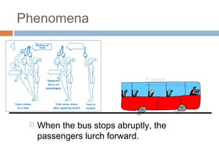
Passengers in a moving bus lean forward when the bus suddenly stops.


Inertia of Direction

The tendency of an object to resist changes in direction.

Example:

Passengers move sideways when a vehicle turns sharply.


Examples of Newton’s First Law

  1. A ball remains stationary until kicked.
  2. A hockey puck slides for a long distance on ice due to minimal friction.
  3. Dust particles fall out when a carpet is shaken.
  4. Passengers fall backward when a bus suddenly starts moving.

These examples demonstrate how objects resist changes in motion.


Newton’s Second Law of Motion

Image
Image
Image
Image

Statement of the Second Law

Newton’s Second Law states:

The rate of change of momentum of an object is directly proportional to the applied force and occurs in the direction of the force.

This law provides the quantitative relationship between force, mass, and acceleration.


Mathematical Expression

Newton’s second law is commonly written as:

[
F = ma
]

Where:

(F) = force
(m) = mass
(a) = acceleration

This equation shows that acceleration is directly proportional to the applied force and inversely proportional to mass.


Momentum and Force

Momentum is defined as:

[
p = mv
]

Where:

(m) = mass
(v) = velocity

Newton originally expressed the second law in terms of momentum:

[
F = \frac{dp}{dt}
]

This means force changes the momentum of an object.


Effects of Force

Force can cause:

  1. Acceleration
  2. Deceleration
  3. Change in direction
  4. Deformation of objects

Example:

When a football is kicked, the applied force changes its velocity.


Applications of Newton’s Second Law

Newton’s second law is widely used in engineering and physics.

Examples include:

Vehicle acceleration
Rocket propulsion
Sports mechanics
Machine design
Structural engineering

For example, a car with a powerful engine produces greater force, resulting in higher acceleration.


Newton’s Third Law of Motion

Image
Image
Image
Image

Statement of the Third Law

Newton’s Third Law states:

For every action, there is an equal and opposite reaction.

This means forces always occur in pairs.


Action and Reaction Forces

When two objects interact:

  • Object A exerts force on object B
  • Object B exerts equal and opposite force on object A

These forces are called action and reaction forces.

Characteristics:

  • Equal magnitude
  • Opposite direction
  • Act on different objects

Examples of Newton’s Third Law

Walking

When a person walks:

  • The foot pushes the ground backward.
  • The ground pushes the person forward.

Rocket Launch

Rocket engines push gases downward.

The gases push the rocket upward.


Swimming

A swimmer pushes water backward.

Water pushes the swimmer forward.


Gun Recoil

When a gun fires a bullet:

  • Bullet moves forward.
  • Gun recoils backward.

Free Body Diagrams

A free body diagram is a diagram used to show all forces acting on an object.

Common forces include:

Weight
Normal force
Friction
Tension
Applied force

Free body diagrams help solve problems involving Newton’s laws.


Types of Forces

Several forces appear in Newtonian mechanics.

Gravitational Force

Attractive force between masses.

Frictional Force

Force opposing motion between surfaces.

Normal Force

Force exerted by surfaces supporting objects.

Tension Force

Force transmitted through strings or cables.

Air Resistance

Force resisting motion through air.


Applications of Newton’s Laws

Newton’s laws are applied in many fields.

Transportation

Design of vehicles and braking systems.

Aerospace Engineering

Rocket launches and spacecraft motion.

Sports Science

Analyzing athlete performance.

Mechanical Engineering

Machine design and structural analysis.

Robotics

Robot movement and control systems.


Limitations of Newton’s Laws

Although Newton’s laws are powerful, they have limitations.

They are not accurate for:

Objects moving close to the speed of light (relativity).

Extremely small particles (quantum mechanics).

For everyday speeds and sizes, however, Newton’s laws work extremely well.


Importance in Physics

Newton’s laws form the basis for many areas of physics.

They are used in:

Mechanics
Engineering physics
Astrophysics
Structural engineering
Vehicle dynamics

Understanding these laws allows scientists and engineers to predict how objects will move under different forces.


Summary

Newton’s laws of motion are three fundamental principles that explain how objects move and interact with forces. The first law describes inertia and explains why objects resist changes in motion. The second law provides the mathematical relationship between force, mass, and acceleration. The third law explains that forces occur in equal and opposite pairs.

Together, these laws provide a powerful framework for analyzing motion and predicting the behavior of physical systems. From everyday activities like walking and driving to complex technologies like rockets and satellites, Newton’s laws remain essential for understanding the physical world.


Tags

Distance, Displacement, Speed, Velocity, and Acceleration

Image
Image
Image
Image

Introduction

In physics, motion is one of the most fundamental phenomena studied in classical mechanics. To understand motion, physicists describe how objects change position with time. Several physical quantities are used to characterize motion, including distance, displacement, speed, velocity, and acceleration. These quantities help explain how far an object travels, how fast it moves, and how its motion changes over time.

Distance and displacement describe how far an object moves. Speed and velocity describe how fast the object moves. Acceleration describes how the velocity changes with time.

These quantities are essential in kinematics, the branch of physics that studies motion without considering the forces causing it. By analyzing these quantities, scientists can predict how objects move in different situations.

For example, when a car travels along a road, we can describe:

  • The total distance the car has traveled
  • The change in position from start to end
  • The rate at which the car moves
  • The direction of motion
  • How quickly the speed changes

Understanding these quantities helps in studying motion in transportation, engineering, sports, robotics, and astronomy.


Distance

Definition of Distance

Distance is the total length of the path traveled by an object during motion.

Distance is a scalar quantity, meaning it has magnitude but no direction.

It tells us how much ground an object has covered, regardless of the direction of motion.

For example, if a person walks 10 meters forward and then 5 meters backward, the total distance traveled is:

[
Distance = 10 + 5 = 15 , m
]

Distance only measures the total path length.


Characteristics of Distance

Distance has several important properties:

  1. It is always positive.
  2. It does not depend on direction.
  3. It depends on the path taken.
  4. It is a scalar quantity.
  5. It is measured in units of length.

The SI unit of distance is meter (m).

Other units include:

Kilometer (km)
Centimeter (cm)
Millimeter (mm)


Examples of Distance

Example 1

A runner completes one lap of a circular track of length 400 meters.

Distance traveled = 400 meters

Example 2

A car moves:

20 km east
10 km west

Distance traveled = 30 km

Even though the directions differ, the total path length is added.


Displacement

Definition of Displacement

Displacement is the shortest straight-line distance between the initial and final positions of an object, along with direction.

Displacement is a vector quantity.

Mathematically:

[
Displacement = Final\ Position – Initial\ Position
]

[
s = x_f – x_i
]

Where:

(x_f) = final position
(x_i) = initial position


Characteristics of Displacement

Displacement has several properties:

  1. It has magnitude and direction.
  2. It is independent of the path taken.
  3. It can be positive, negative, or zero.
  4. It is always the shortest path between two points.

The SI unit of displacement is meter (m).


Examples of Displacement

Example 1

A person walks from point A to point B which is 10 meters east.

Displacement = 10 m east

Example 2

A person walks 10 meters east and then returns to the starting point.

Distance = 20 m
Displacement = 0

Even though motion occurred, the final position is the same as the initial position.


Distance vs Displacement

FeatureDistanceDisplacement
TypeScalarVector
DirectionNot requiredRequired
Path dependencyDepends on pathIndependent of path
SignAlways positiveCan be positive, negative, or zero

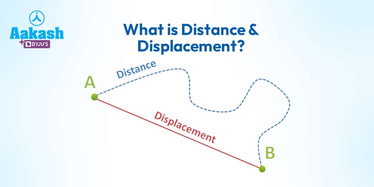
Distance describes how much ground is covered, while displacement describes how far and in what direction an object moved.


Speed

Definition of Speed

Speed is the rate at which distance is covered with respect to time.

[
Speed = \frac{Distance}{Time}
]

Speed is a scalar quantity because it does not involve direction.

The SI unit of speed is:

[
m/s
]

Other common units include:

km/h
cm/s


Average Speed

Average speed is defined as:

[
Average\ Speed = \frac{Total\ Distance}{Total\ Time}
]

Example:

A car travels 120 km in 2 hours.

[
Average\ Speed = \frac{120}{2} = 60 , km/h
]

Average speed gives an overall measure of motion during a journey.


Instantaneous Speed

Instantaneous speed is the speed of an object at a particular moment in time.

For example:

The speedometer of a car shows instantaneous speed.

Instantaneous speed may change continuously during motion.


Uniform Speed

An object has uniform speed if it covers equal distances in equal intervals of time.

Example:

A train moving at a constant speed of 50 km/h.


Non-Uniform Speed

Non-uniform speed occurs when the distance covered in equal intervals of time is different.

Example:

A car moving in city traffic.


Velocity

Image
Image
Image
Image

Definition of Velocity

Velocity is the rate of change of displacement with respect to time.

[
Velocity = \frac{Displacement}{Time}
]

Velocity is a vector quantity because it includes direction.

Example:

Velocity = 20 m/s east

Magnitude = 20 m/s
Direction = east


Average Velocity

Average velocity is defined as:

[
Average\ Velocity = \frac{Total\ Displacement}{Total\ Time}
]

Example:

A person walks:

10 m east
then 10 m west

Displacement = 0

Average velocity = 0


Instantaneous Velocity

Instantaneous velocity is the velocity of an object at a specific moment.

It includes both speed and direction at that instant.


Uniform Velocity

An object has uniform velocity if:

  • Speed remains constant
  • Direction remains constant

Example:

A train moving along a straight track at constant speed.


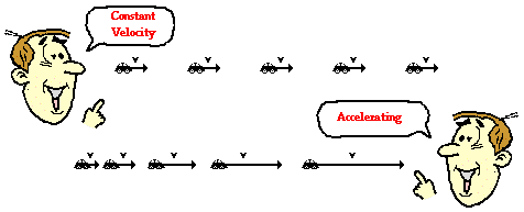
Changing Velocity

Velocity changes when:

  • Speed changes
  • Direction changes
  • Both change

Example:

A car turning around a curve.

Even if speed remains constant, velocity changes because direction changes.


Speed vs Velocity

FeatureSpeedVelocity
Quantity typeScalarVector
Depends onDistanceDisplacement
DirectionNot includedIncluded
SignAlways positiveCan be positive or negative

Speed measures how fast, while velocity measures how fast and in which direction.


Acceleration

Image
Image
Image
Image

Definition of Acceleration

Acceleration is the rate of change of velocity with respect to time.

[
a = \frac{v – u}{t}
]

Where:

(u) = initial velocity
(v) = final velocity
(t) = time

Acceleration is a vector quantity.

The SI unit of acceleration is:

[
m/s^2
]


Types of Acceleration

Uniform Acceleration

Acceleration remains constant.

Example:

Free fall under gravity.


Non-Uniform Acceleration

Acceleration changes with time.

Example:

A car in traffic.


Positive Acceleration

Velocity increases with time.

Example:

A car speeding up.


Negative Acceleration (Deceleration)

Velocity decreases with time.

Example:

Applying brakes.


Graphical Representation of Motion

Distance-Time Graph

A distance-time graph shows how distance changes with time.

Features:

Horizontal line → object at rest
Straight line → uniform speed
Curve → changing speed

Slope of graph:

[
Speed = \frac{Distance}{Time}
]


Velocity-Time Graph

A velocity-time graph shows velocity changes with time.

Slope of graph:

[
Acceleration = \frac{\Delta v}{\Delta t}
]

Area under the graph gives displacement.


Motion with Constant Acceleration

Three important equations describe motion with constant acceleration.

[
v = u + at
]

[
s = ut + \frac{1}{2}at^2
]

[
v^2 = u^2 + 2as
]

These equations are widely used in solving motion problems.


Applications in Real Life

Understanding distance, displacement, speed, velocity, and acceleration is important in many real-world situations.

Transportation

Cars, trains, airplanes, and ships use motion concepts for navigation.

Sports

Athletes analyze speed and acceleration to improve performance.

Engineering

Design of vehicles and machines requires motion analysis.

Astronomy

Planets and satellites move with velocity and acceleration.

Robotics

Robots calculate displacement and velocity to navigate environments.


Importance in Physics

These motion quantities form the foundation of classical mechanics.
They help explain:

Projectile motion
Circular motion
Planetary motion
Newton’s laws of motion
Energy and momentum

Without understanding these quantities, studying advanced physics topics would be difficult.


Summary

Distance, displacement, speed, velocity, and acceleration are fundamental quantities used to describe motion in physics.

Distance measures the total path traveled, while displacement measures the change in position. Speed describes how fast an object moves, while velocity includes both speed and direction. Acceleration describes how velocity changes with time.

Together, these quantities allow scientists and engineers to analyze motion accurately. They play a crucial role in understanding transportation systems, sports performance, engineering designs, and many natural phenomena.

These concepts form the basis for the study of mechanics and are essential for understanding more advanced areas of physics.


Tags

Motion in One Dimension

Image

Image

Image

Image

Introduction

Motion is one of the most fundamental concepts in physics. Everything in the universe—from subatomic particles to galaxies—exhibits motion. The study of motion without considering the forces that cause it is called kinematics, a branch of classical mechanics. Motion in one dimension (1D motion) is the simplest form of motion and serves as the foundation for understanding more complex types of motion.
Motion in one dimension refers to the movement of an object along a single straight line. This line may be horizontal, vertical, or inclined, but the key characteristic is that the object moves only forward or backward along that line. Examples include a car moving along a straight road, a ball falling vertically under gravity, or a train moving along a straight track.

In physics, motion in one dimension is analyzed using quantities such as position, displacement, velocity, speed, and acceleration. Graphical representations and mathematical equations help describe how these quantities change over time.

Understanding one-dimensional motion is essential because it forms the basis for more advanced topics such as two-dimensional motion, projectile motion, circular motion, and dynamics.

1. Fundamental Concepts of Motion

Before studying motion mathematically, it is important to understand the basic quantities used to describe motion.

1.1 Reference Frame

Motion is always described relative to a reference frame. A reference frame is a coordinate system used to measure position and motion.

For example:

  • A person sitting in a train may appear stationary relative to the train.

  • The same person appears moving relative to someone standing on the ground.

Thus motion is relative, meaning it depends on the observer’s frame of reference.

In one-dimensional motion, we usually define a coordinate axis (x-axis) along the direction of motion. The position of the object is then measured along this axis.

1.2 Position

Position describes the location of an object relative to a chosen origin.

If an object lies at point (x) along a straight line, its position is represented as:

[x = \text{position coordinate}]

Example:

  • If a car is 10 meters to the right of the origin, its position is (x = +10) m.

  • If it is 5 meters to the left, its position is (x = -5) m.

The sign indicates direction along the chosen axis.

2. Distance and Displacement

Two important quantities used to describe motion are distance and displacement.

2.1 Distance

Distance is the total path length traveled by an object, regardless of direction.

Characteristics:

  • Scalar quantity

  • Always positive

  • No direction

Example:

A person walks:

  • 5 m forward

  • 3 m backward

Distance = (5 + 3 = 8) m

2.2 Displacement

Displacement is the change in position of an object, including direction.

Mathematically:

[\text{Displacement} = x_f – x_i]

Where:

  • (x_f) = final position

  • (x_i) = initial position

Example:

If a person moves:

  • From 0 m to 5 m

  • Then returns to 2 m

Distance = 8 mDisplacement = (2 – 0 = 2) m

Key differences:

DistanceDisplacement
ScalarVector
Path dependentPath independent
Always positiveCan be positive, negative, or zero

3. Speed and Velocity

Speed and velocity describe how fast an object moves.

3.1 Speed

Speed is the rate at which distance is covered.

[Speed = \frac{Distance}{Time}]

Speed is a scalar quantity.

Example:

If a car travels 100 m in 5 seconds:

[Speed = \frac{100}{5} = 20 , m/s]

Types of speed include:

  • Average speed

  • Instantaneous speed

3.2 Average Speed

Average speed is the total distance traveled divided by total time taken.

[Average\ Speed = \frac{Total\ Distance}{Total\ Time}]

Example:

A car travels:

  • 60 km in 1 hour

  • 40 km in 1 hour

Average speed:

[\frac{100}{2} = 50 , km/h]

3.3 Velocity

Velocity is the rate of change of displacement with respect to time.

[Velocity = \frac{Displacement}{Time}]

Velocity is a vector quantity.

Example:

A car moves:

  • From 0 m to 20 m in 4 s

[Velocity = \frac{20}{4} = 5 , m/s]

Direction matters for velocity.

3.4 Average Velocity

Average velocity is defined as:

[Average\ Velocity = \frac{Total\ Displacement}{Total\ Time}]

Example:

A person walks 10 m east and returns to starting point.

Distance = 20 mDisplacement = 0

Average velocity = 0

Even though motion occurred, displacement is zero.

4. Acceleration

Acceleration measures how quickly velocity changes.

4.1 Definition

Acceleration is the rate of change of velocity with respect to time.

[a = \frac{v – u}{t}]

Where:

  • (u) = initial velocity

  • (v) = final velocity

  • (t) = time

Unit of acceleration:

[m/s^2]

4.2 Types of Acceleration

Uniform Acceleration

Acceleration remains constant.

Example:

Free-falling objects near Earth experience constant acceleration due to gravity.

[g = 9.8 , m/s^2]

Non-uniform Acceleration

Acceleration changes with time.

Example:

A car moving in traffic.

Positive Acceleration

Velocity increases with time.

Negative Acceleration (Deceleration)

Velocity decreases with time.

Example:

Applying brakes in a car.

5. Equations of Motion

For motion with constant acceleration, three important equations describe the relationship between velocity, displacement, acceleration, and time.

First Equation

[v = u + at]

Second Equation

[s = ut + \frac{1}{2}at^2]

Third Equation

[v^2 = u^2 + 2as]

Where:

  • (u) = initial velocity

  • (v) = final velocity

  • (a) = acceleration

  • (s) = displacement

  • (t) = time

These equations are fundamental in solving problems involving one-dimensional motion.

6. Graphical Representation of Motion

Graphs provide a visual way to understand motion.

6.1 Position-Time Graph

Image

Image

Image

Image

A position-time graph shows how position changes with time.

Slope of graph:

[Velocity = \frac{\Delta x}{\Delta t}]

Interpretation:

Horizontal line → object at restStraight line → constant velocityCurve → accelerated motion

6.2 Velocity-Time Graph

Image

Image

Image

Image

A velocity-time graph represents velocity as a function of time.

Key interpretations:

Slope → accelerationArea under graph → displacement

Different patterns:

Horizontal line → constant velocitySloping line → constant accelerationCurve → changing acceleration

7. Free Fall Motion

Free fall is a special case of one-dimensional motion.

When an object falls under gravity alone, the acceleration is constant:

[g = 9.8 , m/s^2]

Equations become:

[v = u + gt]

[s = ut + \frac{1}{2}gt^2]

[v^2 = u^2 + 2gs]

Example:

Dropping a stone from height.

If dropped from rest:

[u = 0]

Then:

[s = \frac{1}{2}gt^2]

8. Relative Motion in One Dimension

Relative motion describes how motion appears to different observers.

If two objects move along the same straight line:

[v_{relative} = v_A – v_B]

Example:

Car A = 60 km/hCar B = 40 km/h

Relative velocity:

[20 , km/h]

If moving in opposite directions:

[v_{relative} = v_A + v_B]

9. Applications of One-Dimensional Motion

Understanding 1D motion helps explain many real-world phenomena.

Transportation

Cars, trains, and elevators often move in straight paths.

Engineering

Designing conveyor belts, lifts, and mechanical systems.

Sports Physics

Motion of runners and sprinters.

Space Science

Rocket launch trajectory begins with vertical motion.

Robotics

Robotic arms moving along linear tracks.

10. Problem-Solving Techniques

To solve motion problems:

Step 1: Identify known quantities

  • Initial velocity

  • Final velocity

  • Time

  • Acceleration

  • Displacement

Step 2: Choose appropriate equation.

Step 3: Substitute values.

Step 4: Solve for unknown.

11. Common Mistakes in Motion Problems

Students often make errors such as:

Ignoring direction signsConfusing distance and displacementUsing wrong equation of motionIncorrect unit conversions

Careful analysis prevents these mistakes.

12. Experimental Study of Motion

Motion can be studied using experimental tools:

Ticker timersMotion sensorsPhotogatesVideo analysis software

These devices measure position and velocity accurately.

13. Limitations of One-Dimensional Motion

Real-world motion rarely occurs strictly in one dimension.

Most motions occur in:

Two dimensions (projectile motion)

Three dimensions (airplane motion)

However, 1D motion is useful as a simplified model.

14. Importance in Physics

Motion in one dimension forms the foundation for many physics topics.

It is essential for understanding:

MechanicsDynamicsNewton’s laws of motionWork and energyMomentumRotational motionWave motion

Mastery of 1D motion allows deeper exploration of classical and modern physics.

15. Summary

Motion in one dimension is the simplest form of motion where an object moves along a straight line. It is analyzed using fundamental quantities such as position, displacement, velocity, speed, and acceleration. Mathematical equations and graphical representations help describe how motion evolves with time.

Key equations such as:

[v = u + at]

[s = ut + \frac{1}{2}at^2]

[v^2 = u^2 + 2as]

allow physicists and engineers to predict motion accurately.

Although simple, the study of one-dimensional motion forms the basis for all of classical mechanics and is essential for understanding the physical world.

Tags

motion in one dimension, straight line motion, kinematics, displacement, distance, velocity, speed, acceleration, equations of motion, uniform acceleration, non uniform acceleration, position time graph, velocity time graph, free fall motion, relative motion, classical mechanics, physics kinematics, linear motion, basic physics motion concepts, motion graphs, kinematic equations

Scalars and Vectors

Image
Image
Image
Image

Introduction

In physics and mathematics, quantities used to describe the physical world are broadly classified into scalars and vectors. These two categories form the foundation of many physical concepts, especially in mechanics, electromagnetism, and engineering. Understanding the difference between scalars and vectors is essential for studying motion, forces, fields, and many other phenomena.

A scalar quantity is completely described by a single numerical value and a unit. It does not involve direction. Examples include temperature, mass, energy, and time.

A vector quantity, on the other hand, requires both magnitude and direction to be fully defined. Examples include displacement, velocity, acceleration, and force.

The distinction between scalars and vectors allows physicists to describe natural phenomena accurately. For example, when describing how fast a car moves, the speed alone is not always sufficient. The direction of motion may also be necessary, which requires the use of vectors.

Vectors are particularly important in physics because many physical processes involve directional effects. Motion, gravitational attraction, electric fields, and magnetic fields are all vector-based phenomena.

This topic is fundamental to understanding many areas of physics, including mechanics, electromagnetism, fluid dynamics, engineering mechanics, and computer graphics.


Scalar Quantities

Definition of Scalar

A scalar is a physical quantity that has magnitude only and no direction.

Mathematically, a scalar can be represented by a single real number.

For example:

Temperature = 30°C
Mass = 5 kg
Time = 10 s

These values describe the quantity completely without requiring direction.

Scalars follow the rules of ordinary algebra.


Characteristics of Scalars

Scalar quantities have several key properties.

  1. They have magnitude only.
  2. They do not require direction.
  3. They can be added or subtracted using normal arithmetic.
  4. They are represented by a single numerical value and unit.
  5. Their values remain unchanged under coordinate rotation.

Because scalars do not depend on direction, they are simpler to work with mathematically compared to vectors.


Examples of Scalar Quantities

Common scalar quantities in physics include:

Mass
Time
Temperature
Energy
Work
Speed
Density
Volume
Pressure
Electric charge
Power
Distance

Each of these quantities can be fully described by a number and unit.

For example:

Mass = 10 kg
Temperature = 25°C
Time = 5 seconds

No directional information is required.


Scalar Operations

Scalars follow the rules of ordinary algebra.

Addition

Two scalar quantities can be added directly.

Example:

5 kg + 3 kg = 8 kg

Subtraction

Example:

10 s − 4 s = 6 s

Multiplication

Example:

Force = mass × acceleration

Even though acceleration is a vector, the multiplication involves scalar magnitude.

Division

Example:

Speed = distance / time

Scalar operations are straightforward because direction does not need to be considered.


Vector Quantities

Definition of Vector

A vector is a physical quantity that has both magnitude and direction.

Vectors cannot be described by magnitude alone.

Example:

Velocity = 20 m/s east

The magnitude is 20 m/s, while the direction is east.

Without direction, the quantity would only represent speed, which is a scalar.


Representation of Vectors

Vectors are usually represented by arrows.

The arrow shows:

Magnitude → length of arrow
Direction → orientation of arrow

Mathematically, vectors are often written using bold letters or arrows.

Examples:

[
\vec{A}
]

or

[
\mathbf{A}
]


Components of a Vector

A vector in two dimensions can be expressed in terms of its components along the x and y axes.

[
\vec{A} = A_x \hat{i} + A_y \hat{j}
]

Where:

(A_x) = horizontal component
(A_y) = vertical component

The magnitude of the vector is:

[
|\vec{A}| = \sqrt{A_x^2 + A_y^2}
]

The direction is given by:

[
\theta = \tan^{-1}\left(\frac{A_y}{A_x}\right)
]

Vector components allow complex motions to be analyzed easily.


Examples of Vector Quantities

Common vector quantities include:

Displacement
Velocity
Acceleration
Force
Momentum
Torque
Electric field
Magnetic field
Gravitational field

Each of these requires both magnitude and direction.

For example:

Force = 10 N north
Velocity = 15 m/s east
Acceleration = 9.8 m/s² downward


Graphical Representation of Vectors

Image
Image
Image
Image

Vectors are often represented graphically using arrows.

Length of Arrow

Represents magnitude.

Direction of Arrow

Represents direction of the vector.

Graphical representation helps visualize vector addition and subtraction.


Vector Addition

Vectors cannot be added using simple arithmetic. Instead, special rules apply.

Two main graphical methods exist for vector addition.


Triangle Law of Vector Addition

In the triangle method:

  1. Place the tail of the second vector at the head of the first vector.
  2. Draw the resultant vector from the tail of the first vector to the head of the second vector.

This resultant represents the combined effect of both vectors.


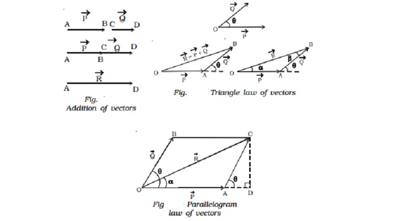
Parallelogram Law of Vector Addition

In this method:

  1. Draw both vectors starting from the same point.
  2. Construct a parallelogram using the two vectors.
  3. The diagonal of the parallelogram represents the resultant vector.

Mathematically:

[
R = \sqrt{A^2 + B^2 + 2AB\cos\theta}
]

Where:

(A) and (B) are vector magnitudes
(\theta) is the angle between them.


Vector Subtraction

Vector subtraction can be performed by adding the negative vector.

[
\vec{A} – \vec{B} = \vec{A} + (-\vec{B})
]

The negative vector has the same magnitude but opposite direction.

Graphically, the reversed vector is added using the triangle method.


Unit Vectors

A unit vector is a vector with magnitude equal to one.

Unit vectors represent direction only.

In a Cartesian coordinate system, the standard unit vectors are:

[
\hat{i}
]

along the x-axis

[
\hat{j}
]

along the y-axis

[
\hat{k}
]

along the z-axis

These unit vectors help express vectors in component form.

Example:

[
\vec{A} = 3\hat{i} + 4\hat{j}
]

Magnitude:

[
|\vec{A}| = \sqrt{3^2 + 4^2} = 5
]


Types of Vectors

Vectors can be categorized into several types.

Zero Vector

A vector with zero magnitude.

Example:

[
\vec{0}
]


Unit Vector

Magnitude equals one.


Equal Vectors

Two vectors with same magnitude and direction.


Negative Vectors

Vectors with equal magnitude but opposite direction.


Parallel Vectors

Vectors pointing in the same or opposite direction.


Collinear Vectors

Vectors lying along the same line.


Scalar and Vector Products

Two important operations between vectors are scalar product and vector product.


Scalar Product (Dot Product)

The dot product between two vectors is defined as:

[
\vec{A} \cdot \vec{B} = AB\cos\theta
]

Result is a scalar.

Applications include:

Work done by a force

[
W = \vec{F} \cdot \vec{d}
]


Vector Product (Cross Product)

The cross product is defined as:

[
\vec{A} \times \vec{B} = AB\sin\theta \hat{n}
]

Result is a vector.

Direction is given by the right-hand rule.

Applications include:

Torque
Magnetic force
Angular momentum


Scalars vs Vectors

FeatureScalarVector
DefinitionMagnitude onlyMagnitude and direction
RepresentationSingle numberArrow
Mathematical operationsOrdinary algebraVector algebra
ExamplesMass, time, temperatureVelocity, force, displacement

Importance in Physics

Scalars and vectors are essential in many branches of physics.

Mechanics

Describing motion and forces.

Electromagnetism

Electric and magnetic fields are vectors.

Fluid Mechanics

Velocity fields in fluids are vector quantities.

Engineering

Structural forces and stresses involve vector analysis.

Computer Graphics

Vectors describe movement and orientation of objects.


Applications in Everyday Life

Vector concepts appear in many real-world situations.

Navigation

Direction and distance of travel.

Weather Forecasting

Wind speed and direction.

Sports

Ball trajectory and player motion.

Aviation

Aircraft velocity and wind vectors.

Robotics

Robot movement and orientation.


Summary

Scalars and vectors are two fundamental types of quantities used in physics to describe the physical world. Scalars represent quantities that have magnitude only, while vectors represent quantities that have both magnitude and direction.

Scalar quantities include mass, temperature, time, and energy, while vector quantities include displacement, velocity, acceleration, and force.

Vectors are represented graphically by arrows and mathematically using vector algebra. Vector addition, subtraction, and multiplication follow special rules that differ from ordinary arithmetic.

Understanding scalars and vectors is crucial for studying motion, forces, and fields in physics. These concepts serve as the building blocks for advanced topics such as mechanics, electromagnetism, and fluid dynamics.


Tags

Motion in Two Dimensions

Image
Image
Image

Introduction

Motion in two dimensions (2D motion) is an important concept in classical mechanics that describes the movement of objects in a plane. Unlike motion in one dimension, where an object moves along a straight line, motion in two dimensions involves movement along two perpendicular axes, typically the x-axis and y-axis. This means that the position of an object must be described using two coordinates rather than one.

Many natural and technological phenomena involve two-dimensional motion. Examples include the motion of a projectile thrown into the air, a football kicked across a field, a bird flying through the sky, or a car turning along a curved road. In these cases, the motion occurs simultaneously in both horizontal and vertical directions.

The study of motion in two dimensions falls under the branch of physics called kinematics, which focuses on describing motion without considering the forces that cause it. By analyzing the components of motion separately along the x and y directions, physicists can simplify complex motion into manageable mathematical relationships.

Understanding two-dimensional motion is essential because it forms the foundation for many advanced topics such as projectile motion, circular motion, orbital mechanics, and vector analysis.


Coordinate System for Two-Dimensional Motion

To analyze motion in two dimensions, a coordinate system is required.

Cartesian Coordinate System

The most commonly used coordinate system is the Cartesian coordinate system, which consists of two perpendicular axes:

  • Horizontal axis (x-axis)
  • Vertical axis (y-axis)

The point where the axes intersect is called the origin (0,0).

The position of an object in two-dimensional space is represented by a coordinate pair:

[
(x, y)
]

Where:

  • (x) represents horizontal position
  • (y) represents vertical position

For example, if an object is located 3 meters to the right and 4 meters upward from the origin, its position is written as:

[
(3,4)
]

This coordinate system allows physicists to track the movement of objects over time.


Position Vector

In two-dimensional motion, position is often expressed using a vector.

A vector quantity has both magnitude and direction.

The position vector is written as:

[
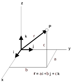
\vec{r} = x\hat{i} + y\hat{j}
]

Where:

  • (x) is the horizontal component
  • (y) is the vertical component
  • (\hat{i}) and (\hat{j}) are unit vectors along the x and y axes

The magnitude of the position vector is given by:

[
|\vec{r}| = \sqrt{x^2 + y^2}
]

This represents the distance from the origin to the object.

Position vectors are extremely useful because they allow motion to be analyzed mathematically in both directions simultaneously.


Displacement in Two Dimensions

Displacement represents the change in position of an object.

If the initial position is:

[
(x_1, y_1)
]

and the final position is:

[
(x_2, y_2)
]

Then the displacement vector is:

[
\vec{s} = (x_2 – x_1)\hat{i} + (y_2 – y_1)\hat{j}
]

The magnitude of displacement is:

[
|\vec{s}| = \sqrt{(x_2 – x_1)^2 + (y_2 – y_1)^2}
]

Unlike distance, displacement depends only on the initial and final positions and not the path taken.


Velocity in Two Dimensions

Velocity in two-dimensional motion describes how quickly the position changes with time.

Velocity is also a vector quantity and can be expressed as:

[
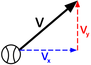
\vec{v} = v_x \hat{i} + v_y \hat{j}
]

Where:

  • (v_x) is the velocity component in the x-direction
  • (v_y) is the velocity component in the y-direction

The magnitude of velocity is:

[
v = \sqrt{v_x^2 + v_y^2}
]

The direction of velocity is given by:

[
\theta = \tan^{-1} \left(\frac{v_y}{v_x}\right)
]

This angle represents the direction of motion relative to the horizontal axis.


Acceleration in Two Dimensions

Acceleration describes how velocity changes with time.

In two-dimensional motion, acceleration also has two components:

[
\vec{a} = a_x \hat{i} + a_y \hat{j}
]

Where:

  • (a_x) is acceleration in the horizontal direction
  • (a_y) is acceleration in the vertical direction

The magnitude of acceleration is:

[
a = \sqrt{a_x^2 + a_y^2}
]

In many physical situations, acceleration may occur in only one direction while velocity exists in both directions.

For example, in projectile motion:

  • Horizontal acceleration is zero
  • Vertical acceleration equals gravitational acceleration

Independent Motion of Components

One of the most important principles in two-dimensional motion is the independence of motion along perpendicular axes.

This means that motion along the x-axis and y-axis can be treated separately.

Horizontal motion and vertical motion do not affect each other.

For example, if a ball is thrown horizontally:

  • Horizontal velocity remains constant
  • Vertical velocity increases due to gravity

This principle simplifies calculations significantly.


Projectile Motion

Image
Image
Image
Image

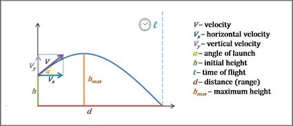
Projectile motion is a special case of two-dimensional motion where an object is thrown into the air and moves under the influence of gravity alone.

Examples include:

  • Throwing a ball
  • Shooting a basketball
  • Launching fireworks
  • Cannonball motion

In projectile motion:

Horizontal motion is uniform.

Vertical motion is uniformly accelerated.


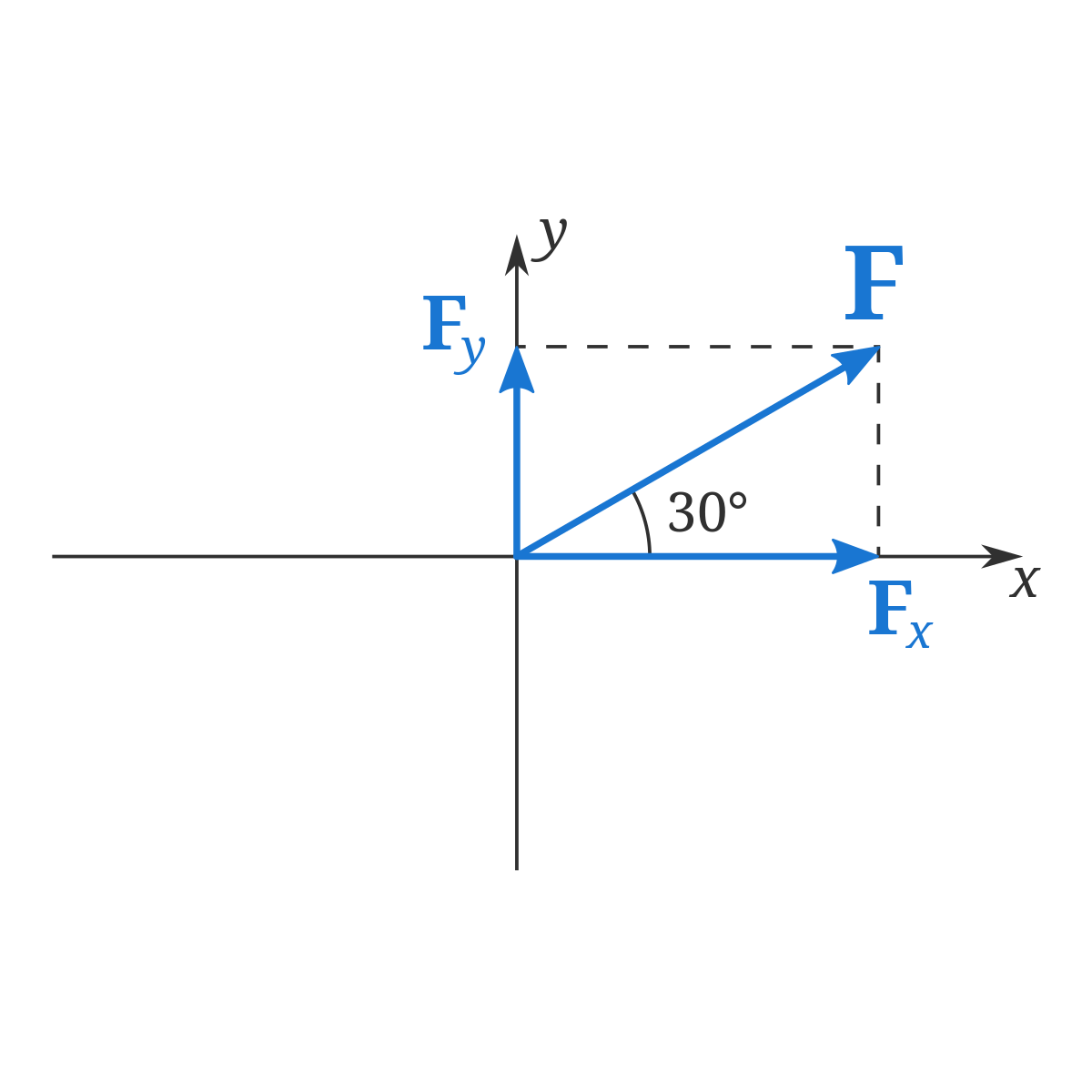
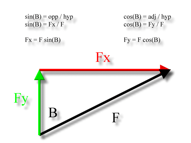
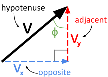
Components of Initial Velocity

When an object is projected with velocity (v_0) at an angle (\theta), the velocity splits into two components.

Horizontal component:

[
v_x = v_0 \cos\theta
]

Vertical component:

[
v_y = v_0 \sin\theta
]

These components determine how the object moves.


Time of Flight

Time of flight is the total time the projectile remains in the air.

[
T = \frac{2 v_0 \sin\theta}{g}
]

Where:

  • (g) is gravitational acceleration.

Maximum Height

The maximum vertical height reached is:

[
H = \frac{v_0^2 \sin^2\theta}{2g}
]

At this point, vertical velocity becomes zero.


Horizontal Range

The horizontal distance traveled is:

[
R = \frac{v_0^2 \sin 2\theta}{g}
]

Maximum range occurs when:

[
\theta = 45^\circ
]


Trajectory of a Projectile

The path followed by a projectile is called its trajectory.

The trajectory is a parabola.

The equation of trajectory is:

[
y = x \tan\theta – \frac{g x^2}{2 v_0^2 \cos^2\theta}
]

This equation shows the curved path of projectile motion.


Relative Motion in Two Dimensions

Relative motion occurs when the motion of one object is observed relative to another moving object.

If two objects move with velocities:

[
\vec{v}_A
]

and

[
\vec{v}_B
]

Then relative velocity is:

[
\vec{v}_{AB} = \vec{v}_A – \vec{v}_B
]

Relative motion is important in:

Navigation

Aircraft motion

River crossing problems


Motion in a Plane

Image
Image
Image
Image

Two-dimensional motion often involves vector addition.

There are two methods for adding vectors:

Triangle Law

Vectors are arranged head-to-tail.

Parallelogram Law

Vectors are drawn from the same origin and the diagonal represents the resultant.

Vector resolution allows a vector to be split into perpendicular components.

This technique is fundamental in analyzing motion.


Circular Motion as Two-Dimensional Motion

Circular motion is also an example of two-dimensional motion.

In circular motion:

  • The object moves in a circular path.
  • Velocity continuously changes direction.

The acceleration directed toward the center is called centripetal acceleration.

[
a_c = \frac{v^2}{r}
]

Where:

  • (v) is velocity
  • (r) is radius

Even if speed is constant, acceleration exists due to the changing direction.


Applications of Two-Dimensional Motion

Two-dimensional motion appears in many real-world situations.

Sports

Ball trajectories in cricket, football, basketball, and golf follow projectile motion.

Engineering

Design of bridges, ramps, and mechanical systems requires motion analysis.

Aerospace

Rocket launches and satellite trajectories involve two-dimensional motion.

Navigation

Ships and aircraft determine relative motion and vector directions.

Robotics

Robot movement across surfaces requires planar motion analysis.


Experimental Study of Two-Dimensional Motion

Physicists study two-dimensional motion using several experimental techniques.

Motion sensors
High-speed cameras
Computer simulations
Trajectory tracking software

These tools allow accurate measurement of position, velocity, and acceleration.


Limitations of Ideal Two-Dimensional Motion

In theoretical physics problems, simplifying assumptions are often made:

Air resistance is ignored.

Gravity is constant.

Earth’s curvature is neglected.

In real-world scenarios, additional factors affect motion.

These include:

Air drag

Wind forces

Variable gravity

Surface friction

More advanced physics models incorporate these effects.


Importance in Physics

Two-dimensional motion plays a crucial role in many fields of physics.

Mechanics

Astrophysics

Engineering physics

Fluid dynamics

Space science

It also forms the basis for understanding three-dimensional motion, where objects move in space along three axes.


Summary

Motion in two dimensions describes the movement of objects in a plane, requiring two coordinates to define position. Unlike one-dimensional motion, objects move simultaneously along horizontal and vertical directions.

The key to understanding two-dimensional motion is breaking vectors into components along the x and y axes. This allows independent analysis of motion along each direction.

Projectile motion is one of the most important examples of two-dimensional motion. It demonstrates how gravity affects vertical motion while horizontal motion remains uniform.

Understanding two-dimensional motion provides essential knowledge for studying many real-world systems, from sports and engineering to aerospace and planetary motion.


Tags

Motion in One Dimension

Image
Image
Image
Image

Introduction

Motion is one of the most fundamental concepts in physics. Everything in the universe—from subatomic particles to galaxies—exhibits motion. The study of motion without considering the forces that cause it is called kinematics, a branch of classical mechanics. Motion in one dimension (1D motion) is the simplest form of motion and serves as the foundation for understanding more complex types of motion.

Motion in one dimension refers to the movement of an object along a single straight line. This line may be horizontal, vertical, or inclined, but the key characteristic is that the object moves only forward or backward along that line. Examples include a car moving along a straight road, a ball falling vertically under gravity, or a train moving along a straight track.

In physics, motion in one dimension is analyzed using quantities such as position, displacement, velocity, speed, and acceleration. Graphical representations and mathematical equations help describe how these quantities change over time.

Understanding one-dimensional motion is essential because it forms the basis for more advanced topics such as two-dimensional motion, projectile motion, circular motion, and dynamics.


1. Fundamental Concepts of Motion

Before studying motion mathematically, it is important to understand the basic quantities used to describe motion.

1.1 Reference Frame

Motion is always described relative to a reference frame. A reference frame is a coordinate system used to measure position and motion.

For example:

  • A person sitting in a train may appear stationary relative to the train.
  • The same person appears moving relative to someone standing on the ground.

Thus motion is relative, meaning it depends on the observer’s frame of reference.

In one-dimensional motion, we usually define a coordinate axis (x-axis) along the direction of motion. The position of the object is then measured along this axis.


1.2 Position

Position describes the location of an object relative to a chosen origin.

If an object lies at point (x) along a straight line, its position is represented as:

[
x = \text{position coordinate}
]

Example:

  • If a car is 10 meters to the right of the origin, its position is (x = +10) m.
  • If it is 5 meters to the left, its position is (x = -5) m.

The sign indicates direction along the chosen axis.


2. Distance and Displacement

Two important quantities used to describe motion are distance and displacement.

2.1 Distance

Distance is the total path length traveled by an object, regardless of direction.

Characteristics:

  • Scalar quantity
  • Always positive
  • No direction

Example:

A person walks:

  • 5 m forward
  • 3 m backward

Distance = (5 + 3 = 8) m


2.2 Displacement

Displacement is the change in position of an object, including direction.

Mathematically:

[
\text{Displacement} = x_f – x_i
]

Where:

  • (x_f) = final position
  • (x_i) = initial position

Example:

If a person moves:

  • From 0 m to 5 m
  • Then returns to 2 m

Distance = 8 m
Displacement = (2 – 0 = 2) m

Key differences:

DistanceDisplacement
ScalarVector
Path dependentPath independent
Always positiveCan be positive, negative, or zero

3. Speed and Velocity

Speed and velocity describe how fast an object moves.

3.1 Speed

Speed is the rate at which distance is covered.

[
Speed = \frac{Distance}{Time}
]

Speed is a scalar quantity.

Example:

If a car travels 100 m in 5 seconds:

[
Speed = \frac{100}{5} = 20 , m/s
]

Types of speed include:

  • Average speed
  • Instantaneous speed

3.2 Average Speed

Average speed is the total distance traveled divided by total time taken.

[
Average\ Speed = \frac{Total\ Distance}{Total\ Time}
]

Example:

A car travels:

  • 60 km in 1 hour
  • 40 km in 1 hour

Average speed:

[
\frac{100}{2} = 50 , km/h
]


3.3 Velocity

Velocity is the rate of change of displacement with respect to time.

[
Velocity = \frac{Displacement}{Time}
]

Velocity is a vector quantity.

Example:

A car moves:

  • From 0 m to 20 m in 4 s

[
Velocity = \frac{20}{4} = 5 , m/s
]

Direction matters for velocity.


3.4 Average Velocity

Average velocity is defined as:

[
Average\ Velocity = \frac{Total\ Displacement}{Total\ Time}
]

Example:

A person walks 10 m east and returns to starting point.

Distance = 20 m
Displacement = 0

Average velocity = 0

Even though motion occurred, displacement is zero.


4. Acceleration

Acceleration measures how quickly velocity changes.

4.1 Definition

Acceleration is the rate of change of velocity with respect to time.

[
a = \frac{v – u}{t}
]

Where:

  • (u) = initial velocity
  • (v) = final velocity
  • (t) = time

Unit of acceleration:

[
m/s^2
]


4.2 Types of Acceleration

Uniform Acceleration

Acceleration remains constant.

Example:

Free-falling objects near Earth experience constant acceleration due to gravity.

[
g = 9.8 , m/s^2
]


Non-uniform Acceleration

Acceleration changes with time.

Example:

A car moving in traffic.


Positive Acceleration

Velocity increases with time.


Negative Acceleration (Deceleration)

Velocity decreases with time.

Example:

Applying brakes in a car.


5. Equations of Motion

For motion with constant acceleration, three important equations describe the relationship between velocity, displacement, acceleration, and time.

First Equation

[
v = u + at
]


Second Equation

[
s = ut + \frac{1}{2}at^2
]


Third Equation

[
v^2 = u^2 + 2as
]

Where:

  • (u) = initial velocity
  • (v) = final velocity
  • (a) = acceleration
  • (s) = displacement
  • (t) = time

These equations are fundamental in solving problems involving one-dimensional motion.


6. Graphical Representation of Motion

Graphs provide a visual way to understand motion.

6.1 Position-Time Graph

Image
Image
Image

A position-time graph shows how position changes with time.

Slope of graph:

[
Velocity = \frac{\Delta x}{\Delta t}
]

Interpretation:

Horizontal line → object at rest
Straight line → constant velocity
Curve → accelerated motion


6.2 Velocity-Time Graph

Image
Image
Image
Image

A velocity-time graph represents velocity as a function of time.

Key interpretations:

Slope → acceleration
Area under graph → displacement

Different patterns:

Horizontal line → constant velocity
Sloping line → constant acceleration
Curve → changing acceleration


7. Free Fall Motion

Free fall is a special case of one-dimensional motion.

When an object falls under gravity alone, the acceleration is constant:

[
g = 9.8 , m/s^2
]

Equations become:

[
v = u + gt
]

[
s = ut + \frac{1}{2}gt^2
]

[
v^2 = u^2 + 2gs
]

Example:

Dropping a stone from height.

If dropped from rest:

[
u = 0
]

Then:

[
s = \frac{1}{2}gt^2
]


8. Relative Motion in One Dimension

Relative motion describes how motion appears to different observers.

If two objects move along the same straight line:

[
v_{relative} = v_A – v_B
]

Example:

Car A = 60 km/h
Car B = 40 km/h

Relative velocity:

[
20 , km/h
]

If moving in opposite directions:

[
v_{relative} = v_A + v_B
]


9. Applications of One-Dimensional Motion

Understanding 1D motion helps explain many real-world phenomena.

Transportation

Cars, trains, and elevators often move in straight paths.

Engineering

Designing conveyor belts, lifts, and mechanical systems.

Sports Physics

Motion of runners and sprinters.

Space Science

Rocket launch trajectory begins with vertical motion.

Robotics

Robotic arms moving along linear tracks.


10. Problem-Solving Techniques

To solve motion problems:

Step 1: Identify known quantities

  • Initial velocity
  • Final velocity
  • Time
  • Acceleration
  • Displacement

Step 2: Choose appropriate equation.

Step 3: Substitute values.

Step 4: Solve for unknown.


11. Common Mistakes in Motion Problems

Students often make errors such as:

Ignoring direction signs
Confusing distance and displacement
Using wrong equation of motion
Incorrect unit conversions

Careful analysis prevents these mistakes.


12. Experimental Study of Motion

Motion can be studied using experimental tools:

Ticker timers
Motion sensors
Photogates
Video analysis software

These devices measure position and velocity accurately.


13. Limitations of One-Dimensional Motion

Real-world motion rarely occurs strictly in one dimension.

Most motions occur in:

Two dimensions (projectile motion)

Three dimensions (airplane motion)

However, 1D motion is useful as a simplified model.


14. Importance in Physics

Motion in one dimension forms the foundation for many physics topics.

It is essential for understanding:

Mechanics
Dynamics
Newton’s laws of motion
Work and energy
Momentum
Rotational motion
Wave motion

Mastery of 1D motion allows deeper exploration of classical and modern physics.


15. Summary

Motion in one dimension is the simplest form of motion where an object moves along a straight line. It is analyzed using fundamental quantities such as position, displacement, velocity, speed, and acceleration. Mathematical equations and graphical representations help describe how motion evolves with time.

Key equations such as:

[
v = u + at
]

[
s = ut + \frac{1}{2}at^2
]

[
v^2 = u^2 + 2as
]

allow physicists and engineers to predict motion accurately.

Although simple, the study of one-dimensional motion forms the basis for all of classical mechanics and is essential for understanding the physical world.


Tags

Mathematical Physics

Image
Image
Image
Image

1. Introduction to Mathematical Physics

Mathematical physics is a branch of science that applies mathematical methods and structures to understand and describe physical phenomena. It serves as a bridge between mathematics and physics, providing the mathematical foundations necessary to formulate physical laws and solve complex problems in nature.

In physics, many phenomena such as motion, heat transfer, electromagnetism, and quantum mechanics can be expressed using mathematical equations. Mathematical physics studies these equations, develops new mathematical techniques, and explores the deep connections between mathematical structures and physical reality.

The subject plays a crucial role in many scientific areas including:

  • Classical mechanics
  • Quantum mechanics
  • Electromagnetism
  • Statistical mechanics
  • Relativity
  • Cosmology
  • Condensed matter physics

Mathematical physics allows scientists to create theoretical models that describe the behavior of physical systems. These models help predict natural phenomena and guide experimental research.

Historically, mathematical physics developed through the work of great scientists such as Isaac Newton, James Clerk Maxwell, Albert Einstein, Paul Dirac, and Richard Feynman.

Today, mathematical physics continues to be a fundamental field for advancing scientific knowledge.


2. Role of Mathematics in Physics

Mathematics is essential in physics because it provides precise tools for describing natural laws.

Key roles of mathematics include:

  • Formulating physical laws
  • Modeling natural systems
  • Solving physical equations
  • Predicting experimental outcomes
  • Analyzing complex systems

Physical theories often begin with observations and experiments. These observations are translated into mathematical equations that describe the relationships between physical quantities.

For example:

Newton’s second law of motion:

F = ma

This equation connects force, mass, and acceleration.

Mathematical physics studies such equations and their implications.


3. Mathematical Models in Physics

A mathematical model represents a physical system using mathematical equations.

Models allow scientists to simulate and predict physical behavior.

Examples include:

  • planetary motion models
  • wave propagation models
  • fluid dynamics equations
  • electromagnetic field equations

Models simplify complex physical systems while retaining essential features.


4. Differential Equations in Physics

Differential equations are one of the most important tools in mathematical physics.

They describe how physical quantities change over time or space.

Examples:

Wave Equation

Describes vibrations and waves.

∂²u/∂t² = c² ∂²u/∂x²

Used in sound waves and water waves.


Heat Equation

Describes heat flow.

∂u/∂t = α ∂²u/∂x²


Schrödinger Equation

Fundamental equation of quantum mechanics.

These equations allow scientists to analyze dynamic systems.


5. Classical Mechanics

Classical mechanics studies motion of objects using mathematical equations.

Two main approaches exist:


Newtonian Mechanics

Based on Newton’s laws.

Key equations include:

F = ma

Used to describe motion of objects on Earth and in space.


Lagrangian Mechanics

Uses energy instead of forces.

Lagrangian:

L = T − V

Where:

T = kinetic energy
V = potential energy


Hamiltonian Mechanics

Another formulation using energy functions.

Hamiltonian:

H = T + V

These methods simplify analysis of complex mechanical systems.


6. Electromagnetism

Electromagnetism describes electric and magnetic fields.

The theory is governed by Maxwell’s equations, which combine electricity and magnetism into a single framework.

Maxwell’s equations describe how electric and magnetic fields interact and propagate as electromagnetic waves.

Applications include:

  • radio waves
  • light
  • microwave technology
  • wireless communication

Mathematical tools such as vector calculus are used to study electromagnetic fields.


7. Quantum Mechanics

Quantum mechanics studies behavior of particles at atomic and subatomic scales.

Unlike classical mechanics, quantum mechanics uses probabilistic models.

The key equation is the Schrödinger equation, which describes the evolution of a particle’s wave function.

Important concepts include:

  • wave-particle duality
  • probability amplitudes
  • quantum states
  • operators and eigenvalues

Quantum mechanics relies heavily on linear algebra and functional analysis.


8. Statistical Mechanics

Statistical mechanics studies large systems of particles.

Instead of tracking each particle individually, statistical methods describe average behavior.

Examples include:

  • temperature
  • pressure
  • entropy

Statistical mechanics connects microscopic particle behavior with macroscopic physical properties.


9. Relativity

Relativity is a theory developed by Albert Einstein.

It describes how space and time behave at high speeds or in strong gravitational fields.

There are two types:


Special Relativity

Deals with motion at speeds close to the speed of light.

Key concept:

Space and time are interconnected.

Equation:

E = mc²


General Relativity

Describes gravity as curvature of spacetime.

Uses differential geometry to model gravitational fields.

General relativity explains phenomena such as:

  • black holes
  • gravitational waves
  • expansion of the universe

10. Mathematical Structures in Physics

Several mathematical tools are widely used in mathematical physics.

Examples include:

  • linear algebra
  • calculus
  • differential equations
  • complex analysis
  • tensor analysis
  • group theory

These tools allow precise modeling of physical systems.


11. Symmetry in Physics

Symmetry plays a crucial role in physical laws.

Symmetry principles help simplify equations and reveal conservation laws.

Example:

Rotational symmetry leads to conservation of angular momentum.

Group theory is often used to analyze symmetries.


12. Conservation Laws

Physical systems often follow conservation laws.

Examples include:

  • conservation of energy
  • conservation of momentum
  • conservation of charge

Mathematical physics studies how these laws arise from symmetries.


13. Wave Phenomena

Waves appear in many areas of physics.
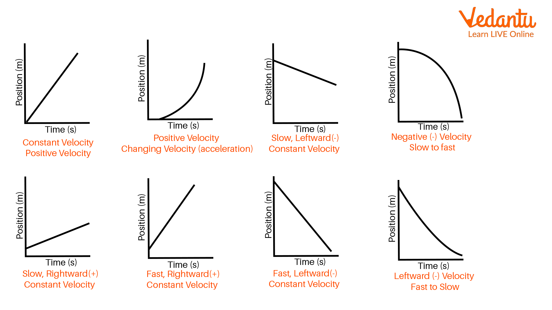
Examples:

  • sound waves
  • light waves
  • water waves
  • quantum waves

Mathematical physics uses wave equations and Fourier analysis to study wave behavior.


14. Field Theory

Field theory studies physical quantities distributed in space.

Examples:

  • electromagnetic fields
  • gravitational fields
  • quantum fields

Fields are represented mathematically as functions of space and time.


15. Mathematical Physics in Engineering

Engineering applications include:

  • electrical circuits
  • signal processing
  • mechanical systems
  • structural analysis

Mathematical models help engineers design and optimize systems.


16. Computational Methods

Modern mathematical physics often relies on computational techniques.

Examples include:

  • numerical simulations
  • finite element methods
  • computational fluid dynamics

These methods solve equations that cannot be solved analytically.


17. Mathematical Physics in Cosmology

Cosmology studies the structure and evolution of the universe.

Mathematical physics helps explain:

  • cosmic expansion
  • dark matter
  • dark energy
  • black holes

Einstein’s field equations describe gravitational effects on a cosmic scale.


18. Mathematical Physics in Quantum Field Theory

Quantum field theory combines quantum mechanics and relativity.

It describes fundamental particle interactions.

Mathematical tools used include:

  • operator theory
  • path integrals
  • symmetry groups

19. Importance of Mathematical Physics

Mathematical physics provides a deep understanding of the laws governing nature.

It allows scientists to:

  • develop physical theories
  • predict experimental results
  • unify different branches of physics

Many modern technologies rely on theories developed in mathematical physics.


20. Modern Developments

Current research areas include:

  • string theory
  • quantum gravity
  • condensed matter physics
  • topological quantum computing

These fields explore fundamental questions about the universe.


Conclusion

Mathematical physics is a powerful interdisciplinary field that combines mathematical rigor with physical insight to describe and understand the natural world. By translating physical phenomena into mathematical equations and models, scientists can analyze complex systems, predict outcomes, and develop new technologies.

From classical mechanics and electromagnetism to quantum mechanics and relativity, mathematical physics provides the theoretical framework for modern science. Its reliance on advanced mathematical tools such as differential equations, linear algebra, and tensor analysis allows researchers to explore deep connections between mathematics and the fundamental laws of nature.

As scientific knowledge continues to advance, mathematical physics remains a cornerstone of theoretical research, helping scientists uncover the underlying structure of the universe and guiding technological innovation.


Tags

Differential Geometry –

Image
Image
Image
Image

1. Introduction to Differential Geometry

Differential geometry is a branch of mathematics that studies the geometry of curves, surfaces, and higher-dimensional spaces using techniques from calculus and linear algebra. The field focuses on analyzing shapes and geometric objects through concepts such as curvature, tangent spaces, and smooth transformations. (Encyclopedia Britannica)

In classical geometry, shapes are often studied using algebraic equations and measurements like lengths and angles. Differential geometry extends these ideas by studying smooth shapes and the way they curve in space. Instead of only considering flat objects such as lines or planes, differential geometry investigates objects that may bend or twist.

Historically, differential geometry developed from the study of curves and surfaces by mathematicians such as Carl Friedrich Gauss and Bernhard Riemann. Gauss introduced the concept of curvature for surfaces, while Riemann extended these ideas to higher-dimensional spaces known as manifolds.

Today, differential geometry is a fundamental area of mathematics with applications in:

  • General relativity
  • Computer graphics
  • Robotics
  • Mechanical engineering
  • Geographical information systems
  • Machine learning
  • Physics and cosmology

By combining geometry with calculus, differential geometry provides tools for understanding the structure of curved spaces and physical systems.


2. Historical Development

The roots of differential geometry go back to ancient geometry and calculus. Early studies of curves began with the work of Isaac Newton and Gottfried Wilhelm Leibniz, who developed calculus in the 17th century.

Gauss and Surface Geometry

Carl Friedrich Gauss studied curved surfaces and introduced Gaussian curvature, showing that curvature can be measured intrinsically without reference to surrounding space.

Riemann and Manifolds

Bernhard Riemann generalized geometry to higher dimensions through the concept of Riemannian manifolds, allowing geometry to be studied on abstract curved spaces.

These developments laid the foundation for modern differential geometry.


3. Curves in Differential Geometry

A curve is one of the simplest objects studied in differential geometry.

Mathematically, a curve can be represented as a function:

γ(t) = (x(t), y(t), z(t))

Where t is a parameter representing position along the curve.

Examples include:

  • Straight lines
  • Circles
  • Spirals
  • Helices

Curves are studied using calculus by analyzing their derivatives.


4. Tangent Vectors and Tangent Lines

A tangent vector describes the direction in which a curve moves at a particular point.

For a curve γ(t):

T = dγ/dt

This vector represents the instantaneous direction of motion.

The tangent vector forms a tangent line, which approximates the curve near the point.

Tangent vectors are fundamental because they allow the geometry of curves to be studied using derivatives.


5. Curvature of Curves

Curvature measures how much a curve deviates from being straight.

For a curve in space:

κ = |dT/ds|

Where:

T = unit tangent vector
s = arc length

If curvature is:

0 → straight line
Large → sharp bending

Curvature describes the geometric behavior of curves.


6. Torsion

While curvature describes bending, torsion measures twisting of a curve in three dimensions.

Torsion describes how a curve moves out of its plane.

Example:

A helix has both curvature and torsion.

These two properties together describe the full geometry of a space curve.


7. Surfaces in Differential Geometry

A surface is a two-dimensional object embedded in three-dimensional space.

Examples include:

  • Sphere
  • Cylinder
  • Torus
  • Paraboloid

Surfaces can be described using parametric equations:

r(u,v)

Where u and v are parameters.

Surfaces extend the study of curves to two dimensions.


8. Tangent Planes

At each point on a smooth surface, there exists a tangent plane.

The tangent plane approximates the surface near that point.

It is defined using partial derivatives:

r_u and r_v

These vectors span the tangent plane.

Tangent planes are essential for analyzing surface geometry.


9. Fundamental Forms

Differential geometry uses two important mathematical objects:

First Fundamental Form

Describes distances and angles on a surface.

It defines the metric of the surface.

Second Fundamental Form

Describes how the surface bends in space.

These two forms together describe the geometry of surfaces.


10. Curvature of Surfaces

Curvature is one of the central ideas in differential geometry.

Two main types exist:

Gaussian Curvature

Measures intrinsic curvature.

Example:

Sphere → positive curvature
Plane → zero curvature
Saddle surface → negative curvature

Mean Curvature

Average curvature of the surface.

Used in minimal surface theory.

Curvature describes how surfaces bend in space.


11. Geodesics

A geodesic is the shortest path between two points on a curved surface. (Wikipedia)

Examples include:

  • Straight lines on a plane
  • Great circles on a sphere

Geodesics generalize the concept of straight lines to curved spaces.

They are extremely important in physics and navigation.


12. Manifolds

A manifold is a space that locally resembles Euclidean space.

Example:

Surface of a sphere.

Although globally curved, small regions look flat.

Manifolds allow geometry to be studied in higher dimensions.

Differential geometry mainly focuses on smooth manifolds.


13. Tangent Spaces

At each point on a manifold, there is a tangent space.

The tangent space contains all possible tangent vectors at that point.

These spaces allow calculus to be applied to manifolds.


14. Riemannian Geometry

Riemannian geometry studies manifolds equipped with a metric tensor.

The metric defines:

  • distances
  • angles
  • curvature

Riemannian geometry generalizes Euclidean geometry to curved spaces.


15. Riemann Curvature Tensor

In higher dimensions, curvature is described using the Riemann curvature tensor, introduced by Riemann. (Wikipedia)

The tensor measures how vectors change when moved around a curved surface.

It provides a complete description of curvature in manifolds.


16. Gauss–Bonnet Theorem

One of the most important results in differential geometry is the Gauss–Bonnet theorem.

It relates curvature to topology.

The theorem states that the integral of curvature over a surface is related to the Euler characteristic of the surface. (Wikipedia)

This result connects geometry with topology.


17. Differential Forms and Tensors

Modern differential geometry uses advanced mathematical tools such as:

  • tensors
  • differential forms
  • vector fields

These objects allow complex geometric structures to be studied systematically.


18. Applications in Physics

Differential geometry is fundamental to modern physics.

General Relativity

Einstein’s theory describes gravity as curvature of spacetime.

Mass and energy bend spacetime geometry.

Quantum Field Theory

Geometry describes particle interactions.

Electromagnetism

Geometric methods simplify Maxwell’s equations.

These applications rely heavily on differential geometry. (Fiveable)


19. Applications in Computer Science

Differential geometry is used in:

  • computer graphics
  • animation
  • shape modeling
  • image processing

It helps model surfaces and curves for digital objects.


20. Applications in Geography and Engineering

Geographical information systems use differential geometry to model Earth’s curved surface and compute distances and routes accurately. (GeeksforGeeks)

Engineering fields use differential geometry to analyze mechanical systems and materials.


21. Modern Developments

Modern research in differential geometry includes:

  • symplectic geometry
  • geometric analysis
  • geometric topology
  • geometric flows

These fields explore advanced structures and dynamic geometric systems.


22. Importance of Differential Geometry

Differential geometry provides tools for understanding curved spaces and geometric structures.

It connects multiple mathematical fields including:

  • calculus
  • linear algebra
  • topology
  • physics

The subject has become central to modern mathematics and science.


Conclusion

Differential geometry is a powerful mathematical discipline that studies curves, surfaces, and higher-dimensional spaces using calculus and algebra. By introducing concepts such as curvature, geodesics, tangent spaces, and manifolds, differential geometry provides a framework for understanding the geometry of smooth shapes and spaces.

The field has evolved significantly since its origins in the work of Gauss and Riemann, expanding to include advanced topics such as Riemannian geometry, curvature tensors, and geometric analysis. These concepts allow mathematicians and scientists to analyze complex geometric structures in both theoretical and applied contexts.

Today, differential geometry plays a crucial role in modern science and technology. It forms the mathematical foundation for Einstein’s theory of general relativity, contributes to computer graphics and robotics, and helps model natural phenomena in physics and engineering.

Understanding differential geometry opens the door to many advanced areas of mathematics and provides powerful tools for exploring the geometry of the universe.


Tags