Author Archives: AI Education

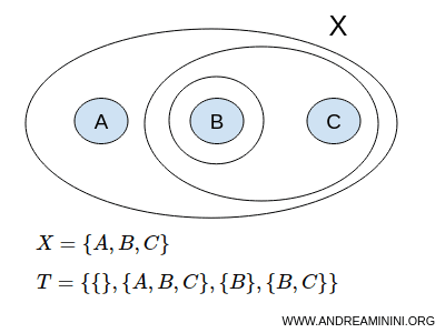
Topology

Image
Image
Image
Image

1. Introduction to Topology

Topology is a branch of mathematics that studies the properties of spaces that remain unchanged under continuous transformations such as stretching, bending, or twisting, but not tearing or gluing. Because of this, topology is often described as “rubber-sheet geometry.”

Unlike classical geometry, which focuses on exact measurements such as angles and distances, topology focuses on qualitative properties such as connectedness, continuity, and the number of holes in a space.

Topology plays a crucial role in modern mathematics and has applications in many areas including:

  • Physics
  • Computer science
  • Robotics
  • Data analysis
  • Cosmology
  • Network theory
  • Artificial intelligence

One famous example used to explain topology is that a coffee cup and a donut (torus) are considered topologically equivalent because each has one hole and can be continuously transformed into the other without cutting.

Topology provides a powerful framework for understanding spaces and shapes in a more abstract and general way.


2. Basic Concepts of Topology

Topology studies mathematical spaces and their properties.

Key concepts include:

  • Topological spaces
  • Open sets
  • Closed sets
  • Continuity
  • Compactness
  • Connectedness

These concepts allow mathematicians to analyze spaces in a generalized way.


3. Topological Spaces

A topological space is a set together with a collection of subsets called open sets.

Formally, a topological space is defined as:

(X, τ)

Where:

X = set of points
τ = topology (collection of open sets)

The topology must satisfy three conditions:

  1. The empty set and the whole set X are open.
  2. Any union of open sets is open.
  3. Any finite intersection of open sets is open.

These rules define the structure of a topological space.


4. Open Sets

An open set is a fundamental concept in topology.

In simple terms, an open set contains none of its boundary points.

Example:

The interval (0,1) in real numbers is an open set.

Open sets help define continuity and convergence.


5. Closed Sets

A closed set contains all its boundary points.

Example:

The interval [0,1] is closed.

Closed sets are complements of open sets.

Properties:

  • Intersection of closed sets is closed.
  • Finite union of closed sets is closed.

6. Interior, Closure, and Boundary

Topology uses several concepts to describe subsets.


Interior

The interior of a set contains all points surrounded entirely by the set.

Example:

Interior of [0,1] is (0,1).


Closure

The closure includes all points of the set plus its boundary.

Example:

Closure of (0,1) is [0,1].


Boundary

Boundary points lie between the set and its complement.

Example:

Boundary of (0,1) is {0,1}.


7. Basis for a Topology

A basis is a collection of open sets used to generate a topology.

Example:

Open intervals form a basis for the topology on real numbers.

Using bases simplifies the description of topological spaces.


8. Subspace Topology

A subspace topology is created when a subset inherits the topology from a larger space.

Example:

Subset of real numbers with induced topology.


9. Continuous Functions

Continuity is a key concept in topology.

A function f is continuous if the preimage of every open set is open.

This definition generalizes continuity from calculus.


10. Homeomorphism

A homeomorphism is a continuous function with a continuous inverse.

Two spaces connected by a homeomorphism are considered topologically equivalent.

Example:

Coffee cup and torus.


11. Connected Spaces

A space is connected if it cannot be divided into two disjoint open sets.

Example:

A single line segment is connected.

Two separate circles form a disconnected space.


12. Path Connectedness

A space is path connected if any two points can be joined by a continuous path.

This concept is stronger than connectedness.


13. Compactness

A set is compact if every open cover has a finite subcover.

Compactness generalizes the idea of closed and bounded sets.

Example:

Closed interval [0,1] is compact.

Compact sets have many important mathematical properties.


14. Metric Spaces

A metric space is a set with a distance function.

Distance function:

d(x,y)

Metric spaces combine topology and geometry.

Example:

Real numbers with standard distance.


15. Topological Manifolds

A manifold is a space that locally resembles Euclidean space.

Examples:

  • surfaces
  • spheres
  • torus

Manifolds are central in modern geometry and physics.


16. Algebraic Topology

Algebraic topology uses algebraic methods to study topological spaces.

Tools include:

  • homology
  • homotopy
  • fundamental groups

These help classify spaces.


17. Fundamental Group

The fundamental group describes loops in a space.

Spaces with different numbers of holes have different fundamental groups.

Example:

Circle has nontrivial fundamental group.


18. Applications of Topology

Topology has many practical applications.


Physics

Used in quantum field theory and cosmology.


Robotics

Topology helps analyze motion planning.


Data Science

Topological data analysis studies patterns in data.


Computer Graphics

Used to model surfaces and shapes.


Network Theory

Topology helps analyze connectivity in networks.


19. Importance of Topology

Topology provides tools for studying spaces in a very general way.

It connects geometry, algebra, and analysis.

Many modern mathematical theories rely on topological ideas.


20. Modern Developments in Topology

Modern topology includes:

  • differential topology
  • algebraic topology
  • geometric topology

These fields study complex structures in mathematics and physics.


Conclusion

Topology is a fascinating branch of mathematics that studies the properties of spaces that remain unchanged under continuous transformations. Unlike classical geometry, which focuses on measurements and distances, topology focuses on the qualitative structure of spaces and how they are connected.

Key concepts such as open sets, closed sets, continuity, compactness, and connectedness provide the foundation for understanding topological spaces. The concept of homeomorphism allows mathematicians to classify spaces based on their fundamental structure rather than their precise geometric shape.

Topology has deep connections with many other branches of mathematics, including algebra, geometry, and analysis. It also has important applications in physics, computer science, robotics, and data science.

As modern science continues to explore complex systems and high-dimensional structures, topology remains an essential tool for understanding the underlying structure of mathematical and physical spaces.


Tags

Abstract Algebra

Image
Image
Image
Image

1. Introduction to Abstract Algebra

Abstract algebra is a branch of mathematics that studies algebraic structures such as groups, rings, fields, and vector spaces. Instead of focusing on specific numbers, abstract algebra studies general mathematical systems defined by operations and rules.
In elementary algebra, we solve equations using numbers and variables. Abstract algebra goes further by studying the underlying structure behind these operations. It investigates how sets of elements behave under operations like addition and multiplication and identifies patterns and properties that apply to many mathematical systems.

Abstract algebra plays a critical role in modern mathematics and has important applications in many scientific fields, including:

  • Cryptography
  • Coding theory
  • Computer science
  • Physics
  • Chemistry
  • Robotics
  • Computer graphics

The foundations of abstract algebra were developed during the 19th century by mathematicians such as Évariste Galois, Niels Henrik Abel, and Emmy Noether, who studied algebraic structures in a systematic way.

Today, abstract algebra is considered one of the core subjects in higher mathematics.


2. Algebraic Structures

An algebraic structure consists of:

  • A set of elements
  • One or more operations defined on that set

The operations must satisfy certain properties.

Examples of algebraic structures include:

  • Groups
  • Rings
  • Fields
  • Vector spaces

These structures help mathematicians study systems in a generalized way.


3. Binary Operations

A binary operation is an operation that combines two elements of a set to produce another element of the same set.

Example:

Addition of integers.

3 + 5 = 8

Both operands and the result belong to the set of integers.

Binary operations must satisfy the closure property, meaning the result remains within the set.


4. Groups

A group is one of the most fundamental structures in abstract algebra.

A group is a set G together with a binary operation satisfying four properties.


Closure

If a and b belong to group G, then:

a * b also belongs to G.


Associativity

(a * b) * c = a * (b * c)


Identity Element

There exists an element e such that:

a * e = a


Inverse Element

For every element a, there exists an inverse a⁻¹ such that:

a * a⁻¹ = e


Example:

The set of integers under addition forms a group.


5. Types of Groups

Groups can be classified based on their properties.


Abelian Group

A group is abelian if the operation is commutative.

a * b = b * a

Example:

Addition of integers.


Non-Abelian Group

A group where the operation is not commutative.

Example:

Matrix multiplication.


Finite Group

A group with a finite number of elements.


Infinite Group

A group with infinitely many elements.

Example:

Integers under addition.


6. Subgroups

A subgroup is a subset of a group that is itself a group under the same operation.

Example:

Even integers form a subgroup of integers.


7. Cyclic Groups

A cyclic group is generated by a single element.

Example:

Multiples of a number under addition.

Example:

G = {0, 2, 4, 6, 8}

Generated by 2.


8. Group Homomorphisms

A homomorphism is a structure-preserving map between groups.

If:

f(a * b) = f(a) * f(b)

Then f is a homomorphism.

Homomorphisms help compare different algebraic structures.


9. Rings

A ring is an algebraic structure consisting of a set equipped with two operations:

  • Addition
  • Multiplication

Properties include:

  • addition forms an abelian group
  • multiplication is associative
  • distributive law holds

Example:

Integers form a ring.


10. Types of Rings


Commutative Ring

Multiplication is commutative.

Example:

Integers.


Non-Commutative Ring

Multiplication is not commutative.

Example:

Matrix rings.


Ring with Identity

Contains multiplicative identity.

Example:

Real numbers.


11. Integral Domains

An integral domain is a commutative ring with no zero divisors.

Example:

Integers.

Zero divisors are elements where:

ab = 0

but neither a nor b is zero.


12. Fields

A field is a ring in which every nonzero element has a multiplicative inverse.

Examples of fields include:

  • Rational numbers
  • Real numbers
  • Complex numbers

Fields allow division (except by zero).


13. Polynomial Rings

Polynomial rings consist of polynomials with coefficients from a ring.

Example:

R[x]

Where R is a ring.

Polynomial rings are important in algebraic geometry.


14. Ideals

An ideal is a special subset of a ring.

Ideals help construct quotient rings.

Example:

Multiples of a number form an ideal.


15. Quotient Rings

A quotient ring is formed by partitioning a ring using an ideal.

Example:

Integers modulo n.


16. Field Extensions

Field extensions expand a field by adding new elements.

Example:

Adding √2 to rational numbers.

Field extensions are important in solving polynomial equations.


17. Galois Theory

Galois theory studies the relationship between polynomial equations and group theory.

It explains why certain equations cannot be solved using radicals.

This theory connects fields and groups.


18. Applications of Abstract Algebra

Abstract algebra has many applications.


Cryptography

Encryption systems use algebraic structures.

Example:

RSA encryption.


Coding Theory

Error-correcting codes rely on algebraic structures.

Used in digital communication.


Computer Science

Used in:

  • algorithms
  • data structures
  • automata theory

Physics

Group theory describes symmetry in physical systems.

Example:

Particle physics.


Robotics

Algebra helps analyze motion and transformations.


19. Importance of Abstract Algebra

Abstract algebra provides a unified framework for studying mathematical structures.

It helps identify patterns and relationships between different mathematical systems.

This field is essential for advanced mathematics and modern scientific research.


Conclusion

Abstract algebra is a powerful branch of mathematics that studies algebraic structures such as groups, rings, and fields. By focusing on the underlying rules and operations that govern mathematical systems, abstract algebra provides a deeper understanding of how different mathematical objects behave.

The study of groups helps analyze symmetry and transformations, while rings and fields provide the foundation for many algebraic systems. Concepts such as homomorphisms, ideals, and field extensions reveal the relationships between different algebraic structures.

Abstract algebra has become increasingly important in modern mathematics and technology, with applications in cryptography, coding theory, computer science, and physics. Its ability to generalize mathematical concepts and uncover hidden patterns makes it one of the most significant areas of higher mathematics.

Understanding abstract algebra not only strengthens mathematical reasoning but also provides tools for solving complex problems in science and engineering.


Tags

Complex Analysis

Image
Image
Image
Image

1. Introduction to Complex Analysis

Complex analysis is a branch of mathematics that studies functions of complex numbers. It extends the ideas of calculus and real analysis into the complex number system. Complex analysis explores the behavior of functions whose variables and values are complex numbers.

Complex analysis is one of the most elegant and powerful areas of mathematics. It provides deep insights into the structure of functions, and many results in complex analysis are stronger and more elegant than their counterparts in real analysis.

The field plays an important role in mathematics, physics, engineering, and applied sciences. Complex analysis is widely used in:

  • Electrical engineering
  • Quantum mechanics
  • Fluid dynamics
  • Signal processing
  • Control theory
  • Electromagnetism
  • Computer graphics

The central idea of complex analysis is studying functions defined on the complex plane, which combines the real and imaginary number systems.


2. Complex Numbers

Complex numbers extend the real numbers by including an imaginary component.

A complex number has the form:

z = a + bi

Where:

a = real part
b = imaginary part
i = imaginary unit

The imaginary unit is defined as:

i² = −1

Example complex numbers:

3 + 2i
−1 + 5i
4 − i


3. Real and Imaginary Parts

For a complex number:

z = a + bi

Real part:

Re(z) = a

Imaginary part:

Im(z) = b

Example:

z = 4 + 7i

Re(z) = 4
Im(z) = 7


4. Complex Plane (Argand Plane)

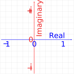
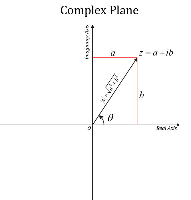
Complex numbers can be represented geometrically on the complex plane.

The horizontal axis represents the real numbers.

The vertical axis represents the imaginary numbers.

Example:

z = 3 + 4i

Point coordinates:

(3,4)

This representation allows complex numbers to be visualized as vectors.


5. Modulus of a Complex Number

The modulus represents the distance of a complex number from the origin.

Formula:

|z| = √(a² + b²)

Example:

z = 3 + 4i

|z| = √(3² + 4²)

|z| = 5


6. Argument of a Complex Number

The argument represents the angle between the positive real axis and the vector representing the complex number.

Notation:

arg(z)

Example:

z = a + bi

Angle:

θ = tan⁻¹(b/a)


7. Polar Form of Complex Numbers

Complex numbers can be written in polar form.

z = r(cosθ + i sinθ)

Where:

r = modulus
θ = argument

Polar form simplifies multiplication and division.


8. Euler’s Formula

One of the most famous formulas in mathematics:

e^(iθ) = cosθ + i sinθ

Using Euler’s formula, complex numbers can be written as:

z = re^(iθ)

This form is called the exponential form.


9. Operations on Complex Numbers

Complex numbers follow standard arithmetic rules.


Addition

(a + bi) + (c + di)

= (a + c) + (b + d)i


Subtraction

(a + bi) − (c + di)

= (a − c) + (b − d)i


Multiplication

(a + bi)(c + di)

= ac + adi + bci + bdi²

Since i² = −1:

= (ac − bd) + (ad + bc)i


Division

Division involves multiplying by the conjugate.


10. Complex Conjugate

The conjugate of a complex number reverses the sign of the imaginary part.

If:

z = a + bi

Then:

z̅ = a − bi

Example:

z = 3 + 4i

z̅ = 3 − 4i

Conjugates help simplify division.


11. Functions of Complex Variables

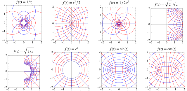
A complex function maps complex numbers to complex numbers.

Example:

f(z) = z²

Where z is complex.

Functions in complex analysis often behave differently from real functions.


12. Limits in Complex Analysis

Limits are defined similarly to real analysis.

lim z→z₀ f(z)

However, in complex analysis the limit must be the same regardless of the direction of approach.


13. Continuity

A function is continuous if:

lim z→z₀ f(z) = f(z₀)

Most elementary complex functions are continuous.


14. Differentiability

A complex function is differentiable if:

f'(z) = lim h→0 [f(z + h) − f(z)] / h

Complex differentiability is stronger than real differentiability.

Functions that are differentiable are called analytic functions.


15. Cauchy-Riemann Equations

For a function:

f(z) = u(x,y) + iv(x,y)

The function is analytic if:

∂u/∂x = ∂v/∂y

∂u/∂y = −∂v/∂x

These equations are fundamental in complex analysis.


16. Analytic Functions

A function is analytic if it is differentiable at every point in a region.

Analytic functions have many remarkable properties.

Examples include:

  • exponential functions
  • trigonometric functions
  • logarithmic functions

17. Complex Integration

Integration in complex analysis involves integrating along curves.

Example:

∮ f(z) dz

This is called contour integration.


18. Cauchy’s Integral Theorem

Cauchy’s theorem states that the integral of an analytic function over a closed contour is zero.

This theorem is one of the most important results in complex analysis.


19. Cauchy’s Integral Formula

Cauchy’s formula allows evaluation of analytic functions inside contours.

It is widely used in theoretical mathematics.


20. Residue Theory

Residue theory helps compute complex integrals using residues at poles.

Residues simplify many difficult integrals.


21. Singularities

Singularities are points where a function is not analytic.

Types include:

  • removable singularities
  • poles
  • essential singularities

22. Applications of Complex Analysis

Complex analysis has many practical applications.


Electrical Engineering

Used in circuit analysis and signal processing.


Fluid Dynamics

Complex functions model fluid flow.


Quantum Mechanics

Complex wave functions describe particles.


Control Systems

Complex analysis helps analyze system stability.


Image Processing

Complex transformations help manipulate images.


23. Importance of Complex Analysis

Complex analysis simplifies many mathematical problems.

It provides elegant solutions and powerful techniques for solving integrals and differential equations.

Many real-world systems rely on complex numbers for modeling physical phenomena.


Conclusion

Complex analysis is a fascinating branch of mathematics that extends the study of functions into the complex number system. By introducing complex numbers and analyzing their properties, mathematicians can explore deeper structures and relationships that are not visible in real analysis.

The study of complex functions reveals remarkable results such as Cauchy’s theorem, Euler’s formula, and residue theory. These concepts provide powerful tools for solving integrals, differential equations, and physical modeling problems.

Complex analysis has significant applications in physics, engineering, and applied mathematics. Its ability to simplify complicated problems and produce elegant solutions makes it one of the most important and beautiful areas of mathematics.

Understanding complex analysis not only strengthens mathematical reasoning but also opens the door to many advanced scientific and engineering applications.


Tags

Real Analysis

Image
Image
Image
Image

1. Introduction to Real Analysis

Real analysis is a branch of mathematics that studies the properties of real numbers, sequences, series, limits, continuity, differentiation, and integration. It provides the rigorous theoretical foundation for calculus and many advanced mathematical concepts.

Real analysis focuses on the structure of the real number system and the behavior of functions defined on real numbers. Unlike basic calculus, which often relies on intuitive ideas, real analysis emphasizes precise definitions, logical reasoning, and mathematical proofs.

The main goal of real analysis is to understand how functions behave and how limits and infinite processes work. It establishes the mathematical rigor behind concepts that appear in calculus, such as limits, derivatives, and integrals.

Real analysis is essential in many areas of mathematics and science, including:

  • Advanced calculus
  • Functional analysis
  • Differential equations
  • Mathematical physics
  • Probability theory
  • Optimization theory
  • Economics and statistics

By studying real analysis, mathematicians gain a deeper understanding of the foundations of mathematical analysis and continuous systems.


2. The Real Number System

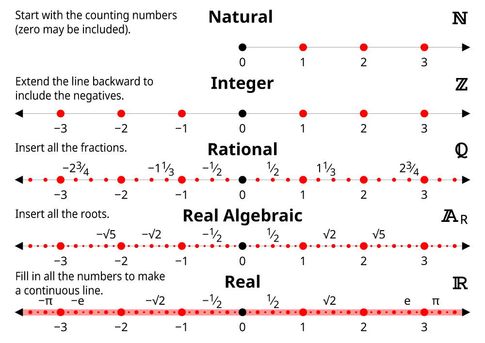
The real numbers form the basis of real analysis.

The set of real numbers is denoted by:

It includes:

  • Natural numbers
  • Integers
  • Rational numbers
  • Irrational numbers

Examples of real numbers:

-3, -1, 0, 1, 2.5, √2, π

The real numbers can be represented on a number line, where every point corresponds to a real number.


3. Properties of Real Numbers

The real numbers satisfy several algebraic properties.


Closure Property

If a and b are real numbers:

a + b is real
a × b is real


Commutative Property

a + b = b + a

a × b = b × a


Associative Property

(a + b) + c = a + (b + c)

(a × b) × c = a × (b × c)


Distributive Property

a(b + c) = ab + ac


4. Order Properties

Real numbers follow an order structure.

If:

a > b

Then a lies to the right of b on the number line.

Properties include:

  • Trichotomy law
  • Transitive property
  • Addition and multiplication inequalities

5. Completeness Property

One of the most important properties of real numbers is completeness.

The completeness property states that every non-empty set of real numbers that is bounded above has a least upper bound (supremum).

This property distinguishes real numbers from rational numbers.

Example:

The set of numbers less than √2 does not have a rational supremum but has a real supremum.


6. Sequences

A sequence is an ordered list of numbers.

Example:

1, 1/2, 1/3, 1/4, …

Sequences are often written as:

{aₙ}

Where n represents the position.


Convergence of Sequences

A sequence converges if its terms approach a fixed value.

Example:

aₙ = 1/n

As n increases, the sequence approaches 0.


Divergent Sequences

If a sequence does not approach a fixed value, it diverges.

Example:

aₙ = n

This sequence grows indefinitely.


7. Limits of Sequences

The limit of a sequence describes the value that sequence approaches.

Definition:

lim n→∞ aₙ = L

Meaning:

As n becomes very large, aₙ approaches L.


Epsilon Definition of Limit

A sequence converges to L if for every ε > 0, there exists N such that:

|aₙ − L| < ε

for all n > N.

This formal definition is fundamental in real analysis.


8. Infinite Series

An infinite series is the sum of infinitely many terms.

Example:

1 + 1/2 + 1/4 + 1/8 + …

If the sum approaches a finite value, the series converges.


Geometric Series

Example:

1 + r + r² + r³ + …

If |r| < 1:

Sum = 1 / (1 − r)


Harmonic Series

1 + 1/2 + 1/3 + 1/4 + …

This series diverges.


9. Functions in Real Analysis

A function is a rule that assigns each element of a set to another element.

Example:

f(x) = x²

Functions are central to real analysis.


10. Limits of Functions

Limits describe how a function behaves near a point.

Example:

lim x→2 (x²)

= 4

Limits help analyze function behavior.


11. Continuity

A function is continuous at point c if:

lim x→c f(x) = f(c)

Graphically, the function has no breaks.

Example:

f(x) = x²

is continuous everywhere.


12. Types of Discontinuities

Functions may have discontinuities.

Examples include:

  • removable discontinuity
  • jump discontinuity
  • infinite discontinuity

13. Differentiation

Differentiation measures the rate of change of a function.

Derivative definition:

f'(x) = lim h→0 [f(x+h) − f(x)] / h

Derivatives describe slopes of curves.


14. Mean Value Theorem

The mean value theorem states that for a continuous function:

There exists a point where the derivative equals the average rate of change.

This theorem is fundamental in analysis.


15. Integration

Integration measures accumulated quantities.

Example:

Area under a curve.

Integral notation:

∫ f(x) dx

Real analysis provides rigorous definitions for integrals.


16. Riemann Integral

The Riemann integral divides a region into small intervals and sums the areas.

It is the standard definition of integration.


17. Uniform Convergence

Uniform convergence describes sequences of functions that converge uniformly.

This concept is important in functional analysis.


18. Metric Spaces

A metric space generalizes the concept of distance.

Distance function:

d(x,y)

Metric spaces extend analysis beyond real numbers.


19. Compactness

A set is compact if every open cover has a finite subcover.

Compact sets have important properties in analysis.


20. Applications of Real Analysis

Real analysis has many applications.


Physics

Used in:

  • quantum mechanics
  • relativity
  • fluid dynamics

Economics

Used in:

  • optimization models
  • economic equilibrium analysis

Engineering

Used in signal processing and control systems.


Probability Theory

Real analysis provides foundations for probability and statistics.


21. Importance of Real Analysis

Real analysis strengthens mathematical rigor.

It explains the theoretical foundations behind calculus.

It also develops logical reasoning and proof techniques.


Conclusion

Real analysis is a fundamental branch of mathematics that provides a rigorous framework for studying real numbers, sequences, limits, and functions. By introducing precise definitions and formal proofs, real analysis establishes the theoretical foundation of calculus and many advanced mathematical disciplines.

Concepts such as convergence, continuity, differentiation, and integration are central to real analysis and help explain the behavior of functions and infinite processes. The field also introduces deeper mathematical ideas such as completeness, metric spaces, and compactness, which extend the study of analysis beyond simple real numbers.

Real analysis plays a critical role in many areas of mathematics, science, and engineering, providing the mathematical tools needed to analyze complex systems and solve real-world problems. Its emphasis on logical rigor and precise reasoning makes it an essential subject for anyone pursuing advanced studies in mathematics.


Tags

Algorithms

Image
Image
Image
Image

1. Introduction to Algorithms

An algorithm is a step-by-step procedure or set of instructions designed to solve a specific problem or perform a particular task. Algorithms are fundamental to computer science and programming because they describe the logic behind how computers process data and perform operations.

In simple terms, an algorithm is like a recipe that tells a computer what to do and in what order to do it. Each algorithm consists of clearly defined steps that lead to a desired output when given certain inputs.

Algorithms are not limited to computer programs; they are used in everyday life as well. For example:

  • Following a recipe to cook a dish
  • Instructions for assembling furniture
  • Steps for solving a mathematical equation
  • Directions for navigating a route on a map

Algorithms play a crucial role in modern technology. They power search engines, social media platforms, navigation systems, artificial intelligence applications, and data analysis tools.


2. Characteristics of an Algorithm

For a procedure to be considered an algorithm, it must satisfy certain characteristics.

Input

An algorithm takes zero or more inputs.

Example:

Numbers provided to perform calculations.


Output

An algorithm produces at least one output.

Example:

The result of a mathematical operation.


Definiteness

Each step must be clearly defined and unambiguous.


Finiteness

The algorithm must terminate after a finite number of steps.


Effectiveness

Every step should be basic enough to be performed exactly and in finite time.


3. Representation of Algorithms

Algorithms can be represented in several ways.


Flowcharts

Flowcharts use graphical symbols to represent algorithm steps.

Common symbols include:

  • Oval (start/end)
  • Rectangle (process)
  • Diamond (decision)

Flowcharts help visualize algorithm logic.


Pseudocode

Pseudocode describes algorithms using a mix of natural language and programming constructs.

Example:

START
Read number
If number is even
   print "Even"
Else
   print "Odd"
END

Programming Languages

Algorithms are implemented using languages such as:

  • Python
  • Java
  • C++
  • JavaScript

4. Types of Algorithms

Algorithms can be classified based on their design and application.


Brute Force Algorithms

Brute force algorithms try all possible solutions until the correct one is found.

Example:

Searching every number in a list.

Advantages:

  • Simple to implement.

Disadvantages:

  • Inefficient for large data.

Divide and Conquer

This technique divides a problem into smaller subproblems, solves them independently, and combines the results.

Examples:

  • Merge sort
  • Quick sort
  • Binary search

Greedy Algorithms

Greedy algorithms make the best choice at each step.

Example:

Selecting the shortest edge in minimum spanning tree algorithms.


Dynamic Programming

Dynamic programming solves complex problems by storing results of subproblems.

Examples:

  • Fibonacci sequence
  • Knapsack problem

Backtracking Algorithms

Backtracking systematically explores all possible solutions.

Example:

Solving puzzles like Sudoku.


5. Searching Algorithms

Searching algorithms find elements within data structures.


Linear Search

Checks every element sequentially.

Example:

Search for number in an array.

Time complexity:

O(n)


Binary Search

Works on sorted arrays.

Process:

Divide array into halves repeatedly.

Time complexity:

O(log n)

Binary search is much faster than linear search.


6. Sorting Algorithms

Sorting algorithms arrange data in a specific order.

Examples include:


Bubble Sort

Repeatedly compares adjacent elements.

Simple but inefficient.

Time complexity:

O(n²)


Selection Sort

Selects the smallest element and swaps it with the first element.


Insertion Sort

Builds sorted list gradually.


Merge Sort

Uses divide-and-conquer.

Time complexity:

O(n log n)


Quick Sort

Highly efficient sorting algorithm.

Average complexity:

O(n log n)


7. Graph Algorithms

Graph algorithms operate on graph structures.

Examples include:


Breadth-First Search (BFS)

Explores vertices level by level.

Used in shortest path problems.


Depth-First Search (DFS)

Explores as far as possible before backtracking.

Used for cycle detection.


Dijkstra’s Algorithm

Finds shortest path in weighted graphs.

Used in navigation systems.


8. Algorithm Complexity

Algorithm complexity measures efficiency.

Two main types:

  • Time complexity
  • Space complexity

Time Complexity

Time complexity measures how long an algorithm takes.

Common complexity classes:

O(1) constant time
O(log n) logarithmic
O(n) linear
O(n log n)
O(n²) quadratic


Space Complexity

Space complexity measures memory usage.

Efficient algorithms use minimal memory.


9. Big-O Notation

Big-O notation describes the upper bound of algorithm complexity.

Example:

Binary search → O(log n)

Bubble sort → O(n²)

Big-O helps compare algorithm efficiency.


10. Recursion in Algorithms

Recursion occurs when a function calls itself.

Example:

Factorial calculation.

n! = n × (n−1)!

Recursion simplifies certain problems but may use more memory.


11. Algorithm Optimization

Optimization improves algorithm efficiency.

Techniques include:

  • reducing unnecessary operations
  • using efficient data structures
  • caching intermediate results

12. Parallel Algorithms

Parallel algorithms execute multiple operations simultaneously.

Used in:

  • supercomputers
  • distributed systems
  • machine learning

13. Randomized Algorithms

Randomized algorithms use randomness in decision-making.

Example:

Randomized quicksort.

They often provide good average performance.


14. Approximation Algorithms

Used when exact solutions are difficult.

Example:

Traveling salesman problem.

Approximation algorithms provide near-optimal solutions.


15. Algorithms in Artificial Intelligence

AI relies heavily on algorithms.

Examples:

  • search algorithms
  • machine learning algorithms
  • optimization techniques

16. Algorithms in Cryptography

Encryption methods use algorithms.

Examples:

  • RSA algorithm
  • AES encryption

These algorithms protect digital data.


17. Algorithms in Data Science

Data science uses algorithms for:

  • data analysis
  • pattern recognition
  • predictive modeling

Machine learning algorithms include:

  • decision trees
  • neural networks
  • clustering algorithms

18. Algorithms in Everyday Life

Algorithms are used in many daily applications.

Examples:

  • Google search ranking
  • GPS navigation
  • recommendation systems
  • online shopping suggestions

19. Importance of Algorithms

Algorithms allow computers to solve problems efficiently.

They help manage large datasets, automate processes, and optimize decision-making.

Without algorithms, modern computing systems would not function effectively.


Conclusion

Algorithms are fundamental to computer science and mathematics, providing systematic methods for solving problems and processing information. From simple tasks such as searching and sorting data to complex operations in artificial intelligence and cryptography, algorithms play a crucial role in modern technology.

Understanding algorithms involves studying their design, efficiency, and implementation. Concepts such as time complexity, recursion, and optimization help developers create faster and more efficient programs. Algorithms are also essential in fields such as machine learning, data science, networking, and cybersecurity.

As technology continues to evolve, the importance of algorithms continues to grow. Efficient algorithms enable faster computation, better decision-making, and improved performance across various applications. Mastering algorithms is therefore essential for anyone interested in computer science, data science, or software engineering.


Tags

Number Theory

Image
Image
Image
Image

1. Introduction to Number Theory

Number theory is a branch of mathematics that studies the properties and relationships of integers. It focuses on understanding the behavior of numbers, particularly whole numbers, and exploring patterns, structures, and relationships among them.

Number theory is often referred to as the “Queen of Mathematics” because of its deep theoretical significance and its connections to many other areas of mathematics.

Historically, number theory was studied for purely theoretical purposes, but today it has many practical applications in fields such as:

  • Cryptography
  • Computer science
  • Coding theory
  • Digital security
  • Data encryption
  • Computer algorithms

Number theory deals with concepts such as:

  • Prime numbers
  • Divisibility
  • Greatest common divisors
  • Modular arithmetic
  • Diophantine equations

These topics allow mathematicians to explore fundamental questions about numbers and their relationships.


2. Integers and Their Properties

The integers are the set of whole numbers, including negative numbers, zero, and positive numbers.

Notation:

ℤ = {…, −3, −2, −1, 0, 1, 2, 3, …}

Integers are the foundation of number theory.

Basic operations on integers include:

  • Addition
  • Subtraction
  • Multiplication
  • Division

However, division is not always possible within integers unless the result is also an integer.


3. Divisibility

Divisibility is one of the most important concepts in number theory.

An integer a divides another integer b if there exists an integer k such that:

b = a × k

Notation:

a | b

Example:

3 | 12

Because:

12 = 3 × 4

If a does not divide b, we write:

a ∤ b


4. Divisibility Rules

Certain rules help determine divisibility.

Examples:

Divisible by 2 → last digit even
Divisible by 3 → sum of digits divisible by 3
Divisible by 5 → last digit 0 or 5
Divisible by 9 → sum of digits divisible by 9

Example:

123

1 + 2 + 3 = 6

6 divisible by 3 → number divisible by 3.


5. Prime Numbers

A prime number is a natural number greater than 1 that has exactly two divisors:

1 and itself.

Examples:

2, 3, 5, 7, 11, 13

Prime numbers are the building blocks of integers.


Composite Numbers

Numbers with more than two factors.

Example:

12 = 2 × 2 × 3

Composite numbers can be expressed as products of primes.


6. Fundamental Theorem of Arithmetic

Every integer greater than 1 can be uniquely expressed as a product of prime numbers.

Example:

60 = 2² × 3 × 5

This factorization is unique.

This theorem is fundamental in number theory.


7. Greatest Common Divisor (GCD)

The greatest common divisor of two integers is the largest integer that divides both numbers.

Example:

GCD(12,18)

Factors of 12:

1,2,3,4,6,12

Factors of 18:

1,2,3,6,9,18

GCD = 6


Euclidean Algorithm

An efficient method for finding GCD.

Example:

GCD(48,18)

48 = 18×2 + 12
18 = 12×1 + 6
12 = 6×2 + 0

GCD = 6


8. Least Common Multiple (LCM)

The least common multiple is the smallest number divisible by both numbers.

Example:

LCM(6,8)

Multiples:

6 → 6,12,18,24
8 → 8,16,24

LCM = 24


9. Modular Arithmetic

Modular arithmetic deals with remainders.

Example:

17 mod 5 = 2

Because:

17 = 5×3 + 2

Modular arithmetic is similar to clock arithmetic.


Congruence

Two numbers are congruent if they have the same remainder.

Notation:

a ≡ b (mod n)

Example:

17 ≡ 2 (mod 5)


10. Applications of Modular Arithmetic

Modular arithmetic is widely used in:

  • cryptography
  • hashing algorithms
  • computer science
  • error detection

11. Euler’s Totient Function

Euler’s function counts numbers less than n that are relatively prime to n.

Notation:

φ(n)

Example:

φ(10)

Numbers less than 10 relatively prime to 10:

1,3,7,9

φ(10) = 4


12. Fermat’s Little Theorem

If p is prime and a is not divisible by p:

a^(p−1) ≡ 1 (mod p)

Example:

2⁴ ≡ 1 (mod 5)

This theorem is widely used in cryptography.


13. Diophantine Equations

Diophantine equations involve integer solutions.

Example:

2x + 3y = 7

Solutions must be integers.

These equations appear in many number theory problems.


14. Perfect Numbers

A perfect number equals the sum of its proper divisors.

Example:

6

Divisors:

1,2,3

Sum:

1 + 2 + 3 = 6


15. Fibonacci Numbers

The Fibonacci sequence appears in number theory.

Sequence:

1,1,2,3,5,8,13…

Each number equals the sum of the previous two.


16. Cryptography and Number Theory

Modern cryptography relies heavily on number theory.

Example:

RSA encryption.

It uses large prime numbers and modular arithmetic.


17. Number Theory in Computer Science

Number theory is used in:

  • hashing algorithms
  • encryption
  • coding theory
  • data security

18. Number Theory in Coding Theory

Coding theory uses number theory for error detection.

Examples:

  • QR codes
  • digital communication systems

19. Advanced Topics in Number Theory

Some advanced topics include:

  • algebraic number theory
  • analytic number theory
  • transcendental numbers
  • prime distribution

These areas explore deeper properties of numbers.


20. Importance of Number Theory

Number theory provides insight into the fundamental nature of numbers.

It has applications in mathematics, cryptography, and computer science.

The study of primes and divisibility has led to important discoveries in modern technology.


Conclusion

Number theory is one of the oldest and most fascinating branches of mathematics, focusing on the study of integers and their properties. From basic concepts such as divisibility and prime numbers to advanced topics like modular arithmetic and Diophantine equations, number theory provides powerful tools for understanding the structure of numbers.

Although number theory was originally developed as a purely theoretical discipline, it now plays a crucial role in modern technology, particularly in cryptography and digital security. The use of prime numbers and modular arithmetic forms the backbone of many encryption systems that protect sensitive information in the digital age.

As mathematical research continues to advance, number theory remains a central area of study, offering deep insights into the patterns and relationships that govern numbers and contributing to developments in computer science, data security, and computational mathematics.


Tags

Combinatorics

Image
Image
Image
Image

1. Introduction to Combinatorics

Combinatorics is a branch of mathematics that deals with counting, arranging, and selecting objects according to specific rules. It focuses on determining how many possible ways events or arrangements can occur.

Combinatorics is fundamental to many areas of mathematics and computer science because it provides tools for analyzing structures, calculating probabilities, and solving complex counting problems.

In everyday life, combinatorics appears in situations such as:

  • Arranging books on a shelf
  • Selecting teams from a group of players
  • Determining possible passwords
  • Calculating lottery outcomes
  • Designing computer algorithms

Combinatorics plays a central role in fields such as:

  • Probability theory
  • Statistics
  • Computer science
  • Cryptography
  • Game theory
  • Network theory
  • Operations research

The study of combinatorics allows mathematicians to analyze patterns and structures efficiently, making it an essential part of discrete mathematics.


2. Basic Principles of Counting

Counting principles form the foundation of combinatorics.

Two important rules are:

  • Addition principle
  • Multiplication principle

Addition Principle

If one task can be performed in m ways and another task can be performed in n ways, and the tasks cannot occur simultaneously, then the total number of ways is:

m + n

Example:

A student can choose a book from:

3 mathematics books
2 physics books

Total choices:

3 + 2 = 5


Multiplication Principle

If a process consists of several steps and each step can occur in multiple ways, the total number of outcomes is the product of the possibilities.

Example:

A password contains:

2 letters and 3 digits.

If letters have 26 possibilities and digits have 10 possibilities:

Total possibilities:

26 × 26 × 10 × 10 × 10


3. Factorials

Factorials are used extensively in combinatorics.

The factorial of a number n is:

n! = n × (n−1) × (n−2) × … × 1

Examples:

5! = 5 × 4 × 3 × 2 × 1 = 120

3! = 3 × 2 × 1 = 6

Special case:

0! = 1

Factorials represent the number of ways objects can be arranged.


4. Permutations

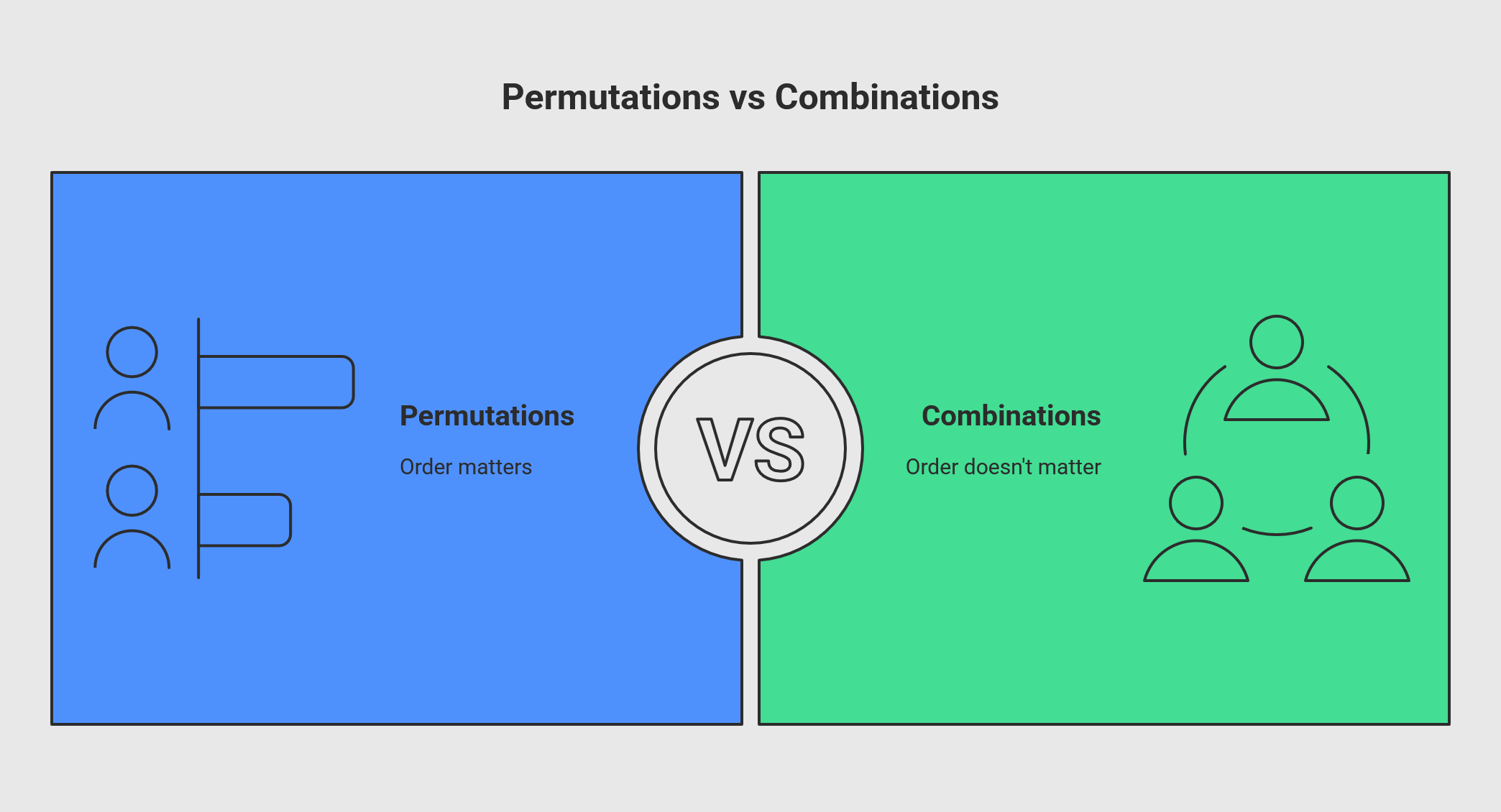
A permutation is an arrangement of objects where order matters.

Example:

Arranging letters A, B, C.

Possible permutations:

ABC
ACB
BAC
BCA
CAB
CBA

Total permutations:

3! = 6


Permutations Formula

If we arrange r objects from n objects:

nPr = n! / (n − r)!

Example:

Number of ways to arrange 3 people from 5.

5P3 = 5! / 2!

= 60


Permutations with Repetition

When repetition is allowed:

Number of permutations:

n^r

Example:

3-digit codes using digits 0–9.

10^3 = 1000


Circular Permutations

Arrangements around a circle.

Formula:

(n − 1)!

Example:

4 people around a table:

3! = 6


5. Combinations

A combination is a selection of objects where order does not matter.

Example:

Selecting 2 students from 4.

Possible selections:

AB
AC
AD
BC
BD
CD


Combination Formula

nCr = n! / (r!(n − r)!)

Example:

Selecting 3 students from 5:

5C3 = 10


6. Differences Between Permutations and Combinations

FeaturePermutationCombination
OrderImportantNot important
ExampleArranging peopleSelecting people

Example:

AB and BA

Permutation: different
Combination: same


7. Binomial Theorem

The binomial theorem expands expressions of the form:

(a + b)^n

Formula:

(a + b)^n = Σ (nCr a^(n−r) b^r)

Example:

(a + b)^3

= a³ + 3a²b + 3ab² + b³

Binomial coefficients appear in Pascal’s triangle.


8. Pascal’s Triangle

Pascal’s triangle is a triangular arrangement of numbers.

Each number is the sum of the two numbers above it.

Example:

1
1 1
1 2 1
1 3 3 1

These numbers represent binomial coefficients.


9. Multiset Combinations

Sometimes elements can repeat.

Example:

Selecting candies from unlimited supply.

Formula:

(n + r − 1)C r


10. Pigeonhole Principle

If more objects than containers exist, at least one container holds multiple objects.

Example:

If 13 people are in a room:

At least two share the same birth month.


11. Inclusion–Exclusion Principle

This principle counts elements in overlapping sets.

Formula:

|A ∪ B| = |A| + |B| − |A ∩ B|

For three sets:

|A ∪ B ∪ C|

= |A| + |B| + |C|

− intersections

  • triple intersection

12. Combinatorial Identities

Important identities include:

nC0 = 1

nCn = 1

nCr = nC(n−r)


13. Generating Functions

Generating functions represent sequences using power series.

Example:

1 + x + x² + x³ + …

They help solve recurrence relations.


14. Recurrence Relations

Recurrence relations define sequences recursively.

Example:

Fibonacci sequence:

F(n) = F(n−1) + F(n−2)


15. Graph Theory and Combinatorics

Graph theory problems often involve combinatorics.

Examples:

  • counting paths
  • network structures
  • graph colorings

16. Combinatorics in Probability

Probability relies heavily on combinatorics.

Example:

Probability of drawing cards from a deck.

Using combinations:

52C5


17. Applications in Computer Science

Combinatorics is used in:

  • algorithm design
  • complexity analysis
  • database indexing
  • cryptography

18. Applications in Cryptography

Secure encryption relies on large combinations and permutations.

Example:

Password security.


19. Applications in Artificial Intelligence

AI algorithms use combinatorial search.

Examples:

  • game playing
  • optimization
  • planning problems

20. Applications in Biology

Combinatorics helps analyze:

  • genetic combinations
  • protein interactions
  • biological networks

21. Applications in Network Design

Network routing problems involve combinatorial optimization.

Examples:

  • traveling salesman problem
  • shortest path problems

22. Importance of Combinatorics

Combinatorics provides powerful techniques for counting and analyzing arrangements.

It forms the foundation for probability theory, computer science, and optimization.

Many modern technologies rely on combinatorial algorithms.


Conclusion

Combinatorics is a vital branch of mathematics that focuses on counting, arranging, and selecting objects according to specific rules. By using principles such as permutations, combinations, factorials, and counting techniques, combinatorics allows mathematicians to analyze complex structures and determine the number of possible outcomes in a system.

The field has wide applications in probability, statistics, computer science, cryptography, and network analysis. Concepts such as Pascal’s triangle, binomial theorem, and the pigeonhole principle provide powerful tools for solving real-world problems involving arrangements and selections.

Combinatorics also plays a critical role in algorithm design and artificial intelligence, where efficient counting and optimization techniques are required. As modern technology continues to rely on large-scale data analysis and complex networks, the importance of combinatorics continues to grow.

Understanding combinatorics helps develop strong analytical and problem-solving skills and provides a foundation for advanced mathematical and computational studies.


Tags

Graph Theory

Image
Image
Image
Image

1. Introduction to Graph Theory

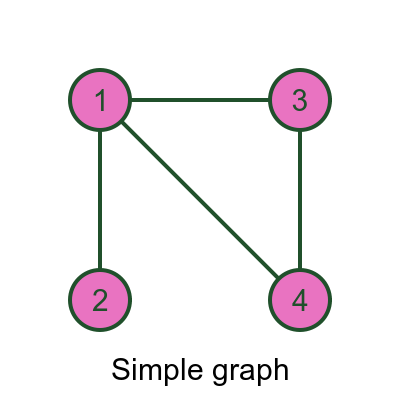
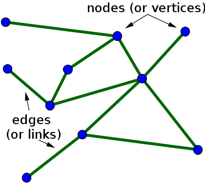
Graph theory is a branch of discrete mathematics that studies graphs, which are mathematical structures used to represent relationships between objects. A graph consists of vertices (nodes) and edges (connections) that link pairs of vertices.

Graph theory is widely used in many fields including computer science, telecommunications, transportation networks, social network analysis, artificial intelligence, and operations research. It helps in modeling systems where objects are connected through relationships.

For example:

  • Cities connected by roads
  • Computers connected in a network
  • People connected in social networks
  • Web pages connected by hyperlinks

All these systems can be represented using graphs.

Graph theory originated in 1736 when the mathematician Leonhard Euler solved the famous Seven Bridges of Königsberg problem, which is considered the first problem in graph theory.

Today, graph theory plays an important role in solving complex problems related to networks, optimization, routing, and data organization.


2. Basic Concepts of Graph Theory

A graph is defined as an ordered pair:

G = (V, E)

Where:

V = set of vertices (nodes)
E = set of edges (connections)

Vertices represent objects, while edges represent relationships between those objects.

Example:

V = {A, B, C}

E = {(A,B), (B,C)}

This graph connects vertex A to B and B to C.


3. Components of a Graph

A graph consists of several components.

Vertices

Vertices (or nodes) represent entities in the graph.

Example:

Cities in a transportation network.


Edges

Edges connect vertices and represent relationships.

Example:

Roads connecting cities.

Edges may be directed or undirected.


4. Types of Graphs

Graphs can be classified based on their properties.


Undirected Graph

Edges have no direction.

Example:

Friendship network.

If A is connected to B, then B is connected to A.


Directed Graph

Edges have direction.

Also called digraphs.

Example:

Twitter followers.

If A follows B, B may not follow A.


Weighted Graph

Edges contain numerical values called weights.

Example:

Distances between cities.


Unweighted Graph

Edges do not have weights.

Only connections matter.


Simple Graph

A graph without loops or multiple edges.


Multigraph

A graph where multiple edges can exist between two vertices.


Complete Graph

Every pair of vertices is connected.

Example:

A complete graph with n vertices has:

n(n−1)/2 edges.


Null Graph

A graph with vertices but no edges.


5. Degree of a Vertex

The degree of a vertex is the number of edges connected to it.

Symbol:

deg(v)

Example:

If vertex A connects to three edges:

deg(A) = 3


Degree in Directed Graphs

Directed graphs have two degrees:

In-degree

Number of incoming edges.

Out-degree

Number of outgoing edges.


6. Paths in Graphs

A path is a sequence of vertices connected by edges.

Example:

A → B → C → D

Path length equals the number of edges.

Paths are important for analyzing connectivity.


7. Cycles

A cycle is a path that starts and ends at the same vertex.

Example:

A → B → C → A

Graphs without cycles are called acyclic graphs.


8. Connected Graphs

A graph is connected if there is a path between every pair of vertices.

If some vertices are isolated, the graph is disconnected.


9. Trees in Graph Theory

A tree is a special type of graph.

Properties:

  • Connected
  • No cycles

Trees are widely used in computer science.

Example:

File system directories.


10. Spanning Trees

A spanning tree connects all vertices of a graph with the minimum number of edges.

If a graph has:

n vertices

A spanning tree has:

n − 1 edges.

Spanning trees are used in network design.


11. Graph Representation

Graphs can be represented in different ways.


Adjacency Matrix

A matrix representing connections.

Example:

If vertex A connects to B:

Matrix entry = 1.


Adjacency List

Each vertex stores a list of its neighbors.

This method saves memory for sparse graphs.


12. Graph Traversal

Graph traversal means visiting all vertices.

Two main algorithms:


Breadth First Search (BFS)

Explores vertices level by level.

Uses a queue.

Applications:

  • shortest path
  • network broadcasting

Depth First Search (DFS)

Explores vertices deeply before backtracking.

Uses stack or recursion.

Applications:

  • cycle detection
  • connectivity analysis

13. Shortest Path Algorithms

Graphs often represent networks where finding the shortest path is important.


Dijkstra’s Algorithm

Finds the shortest path in weighted graphs.

Used in navigation systems.


Bellman-Ford Algorithm

Handles graphs with negative weights.


Floyd-Warshall Algorithm

Finds shortest paths between all vertex pairs.


14. Graph Coloring

Graph coloring assigns colors to vertices so that adjacent vertices have different colors.

Applications include:

  • scheduling problems
  • map coloring
  • register allocation in compilers

15. Bipartite Graphs

A graph is bipartite if vertices can be divided into two sets such that edges connect only between sets.

Example:

Student–course relationship graphs.


16. Planar Graphs

A graph is planar if it can be drawn without edges crossing.

Planar graphs are used in circuit design.


17. Eulerian Graphs

A graph is Eulerian if it contains a path that visits every edge exactly once.

Euler solved the famous Seven Bridges problem using this concept.


18. Hamiltonian Graphs

A Hamiltonian path visits every vertex exactly once.

A Hamiltonian cycle starts and ends at the same vertex.

Used in route optimization problems.


19. Applications of Graph Theory

Graph theory has numerous applications.


Computer Networks

Graph theory models communication networks.

Nodes represent devices.

Edges represent communication links.


Social Networks

Graphs represent relationships between people.

Examples:

  • Facebook friends
  • LinkedIn connections

Transportation Systems

Road networks can be modeled using graphs.

Helps find shortest routes.


Web Search Engines

Search engines use graph algorithms.

Example:

PageRank algorithm.


Biology

Graphs represent biological networks.

Examples:

  • neural networks
  • protein interactions

Artificial Intelligence

Graphs represent knowledge structures.

Used in reasoning systems.


Scheduling Problems

Graph coloring solves scheduling conflicts.

Example:

exam timetables.


20. Importance of Graph Theory

Graph theory provides powerful tools for analyzing networks and relationships.

It helps solve problems involving connectivity, optimization, and routing.

Modern technology relies heavily on graph theory for communication systems, search engines, and social network analysis.


Conclusion

Graph theory is a powerful branch of mathematics that studies networks of connected objects. By representing systems as vertices and edges, graph theory provides a framework for analyzing relationships, connectivity, and structures in complex systems. From simple graphs representing friendships to large networks like the internet, graph theory helps scientists and engineers understand how systems are organized and how they function.

The concepts of paths, cycles, trees, graph traversal, and shortest path algorithms are fundamental tools used in many real-world applications. Graph theory plays a crucial role in computer science, telecommunications, transportation networks, artificial intelligence, and social network analysis.

As technology continues to evolve, the importance of graph theory continues to grow, providing mathematical tools for solving complex network problems and enabling advancements in data analysis, communication systems, and optimization techniques.


Tags

Sets and Relations

Image
Image
Image
Image

1. Introduction to Sets and Relations

Sets and relations are fundamental concepts in mathematics that form the foundation for many advanced topics in algebra, logic, computer science, and data analysis. Set theory provides a systematic way to organize and analyze collections of objects, while relations describe connections between elements of sets.

The concept of sets was introduced by the German mathematician Georg Cantor in the late 19th century. Since then, set theory has become one of the most important frameworks in modern mathematics.

Sets allow mathematicians to represent collections of objects such as numbers, symbols, or even other sets. Relations extend this concept by describing how elements from one set are connected to elements in another set.

These ideas are widely used in fields such as:

  • Mathematics
  • Computer science
  • Database systems
  • Artificial intelligence
  • Logic
  • Statistics
  • Engineering

Understanding sets and relations helps in organizing information, solving mathematical problems, and modeling relationships in real-world systems.


2. Definition of a Set

A set is a well-defined collection of distinct objects.

The objects in a set are called elements or members.

Example:

A = {1, 2, 3, 4}

Here:

1, 2, 3, and 4 are elements of set A.

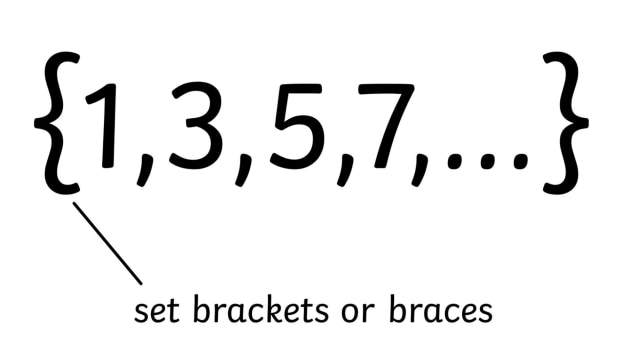
Sets are usually represented using curly braces.


3. Representation of Sets

There are two common ways to represent sets.


Roster Method

Elements are listed explicitly.

Example:

A = {2, 4, 6, 8}


Set Builder Method

Elements are described using a rule.

Example:

A = {x | x is an even number less than 10}

This means the set of even numbers less than 10.


4. Types of Sets

Different types of sets exist depending on their properties.


Empty Set

A set with no elements.

Symbol:

Example:

A = {x | x < 0 and x is natural number}

This set has no elements.


Singleton Set

A set containing only one element.

Example:

{5}


Finite Set

A set with a limited number of elements.

Example:

{1, 2, 3, 4}


Infinite Set

A set with unlimited elements.

Example:

Natural numbers:

{1, 2, 3, …}


Equal Sets

Two sets are equal if they contain the same elements.

Example:

A = {1, 2, 3}

B = {3, 2, 1}

A = B


Equivalent Sets

Sets with the same number of elements.

Example:

A = {1,2,3}

B = {a,b,c}


Universal Set

The universal set contains all elements under consideration.

Symbol:

U

Example:

If studying numbers 1–10:

U = {1,2,3,4,5,6,7,8,9,10}


5. Subsets

A subset is a set whose elements are all contained within another set.

Symbol:

Example:

A = {1,2,3}

B = {1,2}

B ⊆ A


Proper Subset

A subset that is not equal to the original set.

Symbol:

Example:

{1,2} ⊂ {1,2,3}


6. Power Set

The power set of a set is the set of all subsets of that set.

If set A has n elements:

Power set contains:

2ⁿ subsets.

Example:

A = {1,2}

Power set:

{ ∅, {1}, {2}, {1,2} }


7. Operations on Sets

Set operations combine sets in various ways.


Union

The union of two sets includes all elements in either set.

Symbol:

A ∪ B

Example:

A = {1,2,3}

B = {3,4,5}

A ∪ B = {1,2,3,4,5}


Intersection

Intersection includes elements common to both sets.

Symbol:

A ∩ B

Example:

A ∩ B = {3}


Difference

Difference includes elements in one set but not the other.

Symbol:

A − B

Example:

A − B = {1,2}


Complement

Complement includes elements not in the set.

Symbol:

A’

Example:

If universal set:

U = {1,2,3,4,5}

A = {1,2}

A’ = {3,4,5}


8. Venn Diagrams

Venn diagrams visually represent sets and their relationships.

They use circles to represent sets and show intersections, unions, and differences.

Venn diagrams are widely used in probability, statistics, and logic.


9. Cartesian Product

The Cartesian product combines two sets to form ordered pairs.

Symbol:

A × B

Example:

A = {1,2}

B = {a,b}

A × B =

{(1,a), (1,b), (2,a), (2,b)}


10. Relations

A relation is a connection between elements of two sets.

A relation from set A to set B is a subset of the Cartesian product A × B.

Example:

A = {1,2}

B = {a,b}

Relation:

R = {(1,a), (2,b)}


11. Domain and Range

For a relation:

Domain = set of first elements.

Range = set of second elements.

Example:

R = {(1,a),(2,b)}

Domain = {1,2}

Range = {a,b}


12. Types of Relations

Relations have different properties.


Reflexive Relation

Every element relates to itself.

Example:

R = {(1,1),(2,2),(3,3)}


Symmetric Relation

If (a,b) is in relation, then (b,a) is also.

Example:

Friendship relation.


Transitive Relation

If (a,b) and (b,c) exist, then (a,c) exists.

Example:

Ancestor relationships.


13. Equivalence Relations

A relation is an equivalence relation if it is:

  • Reflexive
  • Symmetric
  • Transitive

Example:

Equality relation.


14. Equivalence Classes

Equivalence relations divide sets into groups called equivalence classes.

Example:

Integers grouped by remainder when divided by 3.


15. Functions as Special Relations

A function is a special type of relation.

Each element of the domain maps to exactly one element of the range.

Example:

f(x) = x²


16. Relations in Graph Theory

Relations can be represented using graphs.

Nodes represent elements.

Edges represent relationships.

Used in social networks and communication systems.


17. Applications of Sets

Set theory is used in:

  • probability theory
  • database design
  • computer algorithms
  • artificial intelligence
  • data classification

18. Applications of Relations

Relations help model real-world connections.

Examples include:

  • social networks
  • family trees
  • database relationships
  • network communication

19. Sets and Relations in Computer Science

Computer science uses sets for:

  • data structures
  • database queries
  • programming logic
  • algorithm design

Relations are used in:

  • relational databases
  • graph theory
  • network modeling

20. Importance of Sets and Relations

Sets and relations provide powerful mathematical tools for organizing and analyzing data.

They help describe relationships between objects and simplify complex systems.

Without these concepts, many fields such as computer science, artificial intelligence, and database management would not exist.


Conclusion

Sets and relations form the backbone of modern mathematics and provide essential tools for organizing information and describing relationships between objects. Sets allow mathematicians to define collections of elements and perform operations such as union, intersection, and complement. Relations extend this concept by establishing connections between elements of different sets, enabling the study of structures such as functions, equivalence relations, and mappings.

These concepts are widely applied in many disciplines including mathematics, computer science, data analysis, and engineering. From database systems and network models to probability theory and logic, sets and relations play a crucial role in representing and analyzing complex systems.

Understanding sets and relations is essential for anyone studying mathematics, computer science, or data science because they form the foundation for many advanced topics such as functions, graph theory, and formal logic.


Tags

Logic and Propositions

Image
Image
Image
Image

1. Introduction to Logic and Propositions

Logic is one of the most fundamental branches of mathematics and philosophy. It deals with reasoning, argument structure, and determining whether statements are true or false. Logic forms the foundation for mathematical proofs, computer programming, artificial intelligence, digital circuits, and many scientific disciplines.

A central concept in logic is the proposition, which is a statement that can either be true or false, but not both simultaneously. Propositions allow us to analyze reasoning systematically and determine the validity of arguments.

Logic is widely used in many areas, including:

  • Mathematics
  • Computer science
  • Philosophy
  • Artificial intelligence
  • Digital electronics
  • Data science
  • Linguistics
  • Formal verification

By studying logic and propositions, we develop the ability to analyze statements, construct proofs, and evaluate arguments rigorously.


2. What is a Proposition?

A proposition is a declarative statement that has a definite truth value: either true or false.

Examples of propositions:

  • “2 + 3 = 5”
  • “The Earth revolves around the Sun”
  • “7 is a prime number”

Each of these statements can be evaluated as either true or false.

Examples that are not propositions:

  • “What time is it?”
  • “Close the door”
  • “x + 5 = 10”

The first two are questions or commands. The third contains a variable whose truth depends on the value of x.

Therefore, a proposition must have a definite truth value.


3. Truth Values

Every proposition has a truth value.

Truth values are usually represented by:

T = True
F = False

Example:

p: “5 > 3”

Truth value: True

Another example:

q: “4 is an odd number”

Truth value: False

Truth values form the basis of logical reasoning.


4. Simple and Compound Propositions

Propositions can be classified into two types:

Simple (Atomic) Propositions

These are basic propositions that cannot be broken down into smaller statements.

Example:

p: “It is raining.”

q: “The temperature is 25°C.”


Compound Propositions

Compound propositions are formed by combining simple propositions using logical connectives.

Example:

“It is raining and cold.”

This combines two simple propositions.


5. Logical Connectives

Logical connectives combine propositions to create compound statements.

The most common logical connectives are:

  • NOT
  • AND
  • OR
  • IMPLICATION
  • BICONDITIONAL

Negation (NOT)

Negation reverses the truth value of a proposition.

Symbol:

¬p

Example:

p: “It is raining.”

¬p: “It is not raining.”

Truth table:

p | ¬p
T | F
F | T


Conjunction (AND)

Conjunction combines two propositions and is true only if both are true.

Symbol:

p ∧ q

Example:

p: “It is raining.”

q: “It is cold.”

Compound statement:

“It is raining and cold.”

Truth table:

p | q | p ∧ q
T | T | T
T | F | F
F | T | F
F | F | F


Disjunction (OR)

Disjunction is true if at least one proposition is true.

Symbol:

p ∨ q

Truth table:

p | q | p ∨ q
T | T | T
T | F | T
F | T | T
F | F | F


Implication (IF–THEN)

Implication represents conditional statements.

Symbol:

p → q

Meaning:

“If p is true, then q must be true.”

Truth table:

p | q | p → q
T | T | T
T | F | F
F | T | T
F | F | T


Biconditional

Symbol:

p ↔ q

Meaning:

p is true if and only if q is true.

Truth table:

p | q | p ↔ q
T | T | T
T | F | F
F | T | F
F | F | T


6. Truth Tables

A truth table is a table that shows the truth values of logical expressions for all possible combinations of inputs.

Truth tables help evaluate logical expressions and verify logical equivalences.

Example:

Expression:

p ∧ q

Truth table lists all possible values of p and q.


7. Logical Equivalence

Two statements are logically equivalent if they always have the same truth values.

Example:

p → q is equivalent to ¬p ∨ q

Logical equivalence is useful in simplifying logical expressions.


8. Laws of Logic

Several laws govern logical expressions.


Identity Laws

p ∧ T = p
p ∨ F = p


Domination Laws

p ∨ T = T
p ∧ F = F


Idempotent Laws

p ∨ p = p
p ∧ p = p


Double Negation

¬(¬p) = p


Commutative Laws

p ∧ q = q ∧ p
p ∨ q = q ∨ p


Associative Laws

(p ∧ q) ∧ r = p ∧ (q ∧ r)


Distributive Laws

p ∧ (q ∨ r) = (p ∧ q) ∨ (p ∧ r)


De Morgan’s Laws

¬(p ∧ q) = ¬p ∨ ¬q

¬(p ∨ q) = ¬p ∧ ¬q

These laws are extremely important in logic and computer science.


9. Tautologies and Contradictions

Logical expressions can be classified based on their truth values.


Tautology

A statement that is always true.

Example:

p ∨ ¬p


Contradiction

A statement that is always false.

Example:

p ∧ ¬p


Contingency

A statement that is sometimes true and sometimes false.

Example:

p ∧ q


10. Logical Arguments

Logic is used to evaluate arguments.

An argument consists of:

Premises
Conclusion

Example:

Premise 1: If it rains, the ground is wet.
Premise 2: It is raining.

Conclusion: The ground is wet.

This argument is logically valid.


11. Predicate Logic

Propositional logic deals with whole statements.

Predicate logic extends this by including variables.

Example:

P(x): “x is a prime number.”


12. Quantifiers

Quantifiers describe how many objects satisfy a predicate.


Universal Quantifier

Symbol:

Meaning:

“For all”

Example:

∀x (x + 0 = x)


Existential Quantifier

Symbol:

Meaning:

“There exists”

Example:

∃x (x² = 4)


13. Logic in Mathematics

Logic is the foundation of mathematical proofs.

Types of proofs include:

  • Direct proof
  • Proof by contradiction
  • Proof by contrapositive
  • Mathematical induction

14. Logic in Computer Science

Logic is essential in programming and computing.

Applications include:

  • algorithm design
  • program verification
  • database queries
  • artificial intelligence

Programming languages use logical operators like:

AND, OR, NOT.


15. Logic in Digital Electronics

Digital circuits use logical operations.

Examples include:

  • AND gate
  • OR gate
  • NOT gate
  • NAND gate
  • NOR gate

Computers operate using binary logic.


16. Logic in Artificial Intelligence

AI systems use logical reasoning to make decisions.

Example applications:

  • expert systems
  • automated reasoning
  • knowledge representation

17. Logic in Linguistics

Logic helps analyze sentence structure and meaning.

Used in:

  • semantic analysis
  • natural language processing

18. Importance of Logic

Logic helps people:

  • think clearly
  • evaluate arguments
  • avoid fallacies
  • build valid proofs

It is essential for scientific reasoning and critical thinking.


Conclusion

Logic and propositions form the foundation of reasoning in mathematics, computer science, and philosophy. Propositions provide the basic units of logical analysis, while logical connectives allow complex statements to be constructed and evaluated. Through truth tables, logical laws, and equivalence rules, logic enables systematic analysis of arguments and statements.

The study of logic extends beyond mathematics into many practical fields, including computer programming, artificial intelligence, digital circuit design, and formal verification systems. Predicate logic further expands the power of logical reasoning by introducing variables and quantifiers, allowing more detailed and flexible analysis of statements.

Understanding logic and propositions is essential for anyone interested in mathematics, computer science, or analytical reasoning. By mastering logical principles, individuals can improve their problem-solving skills, construct valid arguments, and develop a deeper understanding of formal systems.


Tags