


1. Introduction to Mathematical Physics
Mathematical physics is a branch of science that applies mathematical methods and structures to understand and describe physical phenomena. It serves as a bridge between mathematics and physics, providing the mathematical foundations necessary to formulate physical laws and solve complex problems in nature.
In physics, many phenomena such as motion, heat transfer, electromagnetism, and quantum mechanics can be expressed using mathematical equations. Mathematical physics studies these equations, develops new mathematical techniques, and explores the deep connections between mathematical structures and physical reality.
The subject plays a crucial role in many scientific areas including:
- Classical mechanics
- Quantum mechanics
- Electromagnetism
- Statistical mechanics
- Relativity
- Cosmology
- Condensed matter physics
Mathematical physics allows scientists to create theoretical models that describe the behavior of physical systems. These models help predict natural phenomena and guide experimental research.
Historically, mathematical physics developed through the work of great scientists such as Isaac Newton, James Clerk Maxwell, Albert Einstein, Paul Dirac, and Richard Feynman.
Today, mathematical physics continues to be a fundamental field for advancing scientific knowledge.
2. Role of Mathematics in Physics
Mathematics is essential in physics because it provides precise tools for describing natural laws.
Key roles of mathematics include:
- Formulating physical laws
- Modeling natural systems
- Solving physical equations
- Predicting experimental outcomes
- Analyzing complex systems
Physical theories often begin with observations and experiments. These observations are translated into mathematical equations that describe the relationships between physical quantities.
For example:
Newton’s second law of motion:
F = ma
This equation connects force, mass, and acceleration.
Mathematical physics studies such equations and their implications.
3. Mathematical Models in Physics
A mathematical model represents a physical system using mathematical equations.
Models allow scientists to simulate and predict physical behavior.
Examples include:
- planetary motion models
- wave propagation models
- fluid dynamics equations
- electromagnetic field equations
Models simplify complex physical systems while retaining essential features.
4. Differential Equations in Physics
Differential equations are one of the most important tools in mathematical physics.
They describe how physical quantities change over time or space.
Examples:
Wave Equation
Describes vibrations and waves.
∂²u/∂t² = c² ∂²u/∂x²
Used in sound waves and water waves.
Heat Equation
Describes heat flow.
∂u/∂t = α ∂²u/∂x²
Schrödinger Equation
Fundamental equation of quantum mechanics.
These equations allow scientists to analyze dynamic systems.
5. Classical Mechanics
Classical mechanics studies motion of objects using mathematical equations.
Two main approaches exist:
Newtonian Mechanics
Based on Newton’s laws.
Key equations include:
F = ma
Used to describe motion of objects on Earth and in space.
Lagrangian Mechanics
Uses energy instead of forces.
Lagrangian:
L = T − V
Where:
T = kinetic energy
V = potential energy
Hamiltonian Mechanics
Another formulation using energy functions.
Hamiltonian:
H = T + V
These methods simplify analysis of complex mechanical systems.
6. Electromagnetism
Electromagnetism describes electric and magnetic fields.
The theory is governed by Maxwell’s equations, which combine electricity and magnetism into a single framework.
Maxwell’s equations describe how electric and magnetic fields interact and propagate as electromagnetic waves.
Applications include:
- radio waves
- light
- microwave technology
- wireless communication
Mathematical tools such as vector calculus are used to study electromagnetic fields.
7. Quantum Mechanics
Quantum mechanics studies behavior of particles at atomic and subatomic scales.
Unlike classical mechanics, quantum mechanics uses probabilistic models.
The key equation is the Schrödinger equation, which describes the evolution of a particle’s wave function.
Important concepts include:
- wave-particle duality
- probability amplitudes
- quantum states
- operators and eigenvalues
Quantum mechanics relies heavily on linear algebra and functional analysis.
8. Statistical Mechanics
Statistical mechanics studies large systems of particles.
Instead of tracking each particle individually, statistical methods describe average behavior.
Examples include:
- temperature
- pressure
- entropy
Statistical mechanics connects microscopic particle behavior with macroscopic physical properties.
9. Relativity
Relativity is a theory developed by Albert Einstein.
It describes how space and time behave at high speeds or in strong gravitational fields.
There are two types:
Special Relativity
Deals with motion at speeds close to the speed of light.
Key concept:
Space and time are interconnected.
Equation:
E = mc²
General Relativity
Describes gravity as curvature of spacetime.
Uses differential geometry to model gravitational fields.
General relativity explains phenomena such as:
- black holes
- gravitational waves
- expansion of the universe
10. Mathematical Structures in Physics
Several mathematical tools are widely used in mathematical physics.
Examples include:
- linear algebra
- calculus
- differential equations
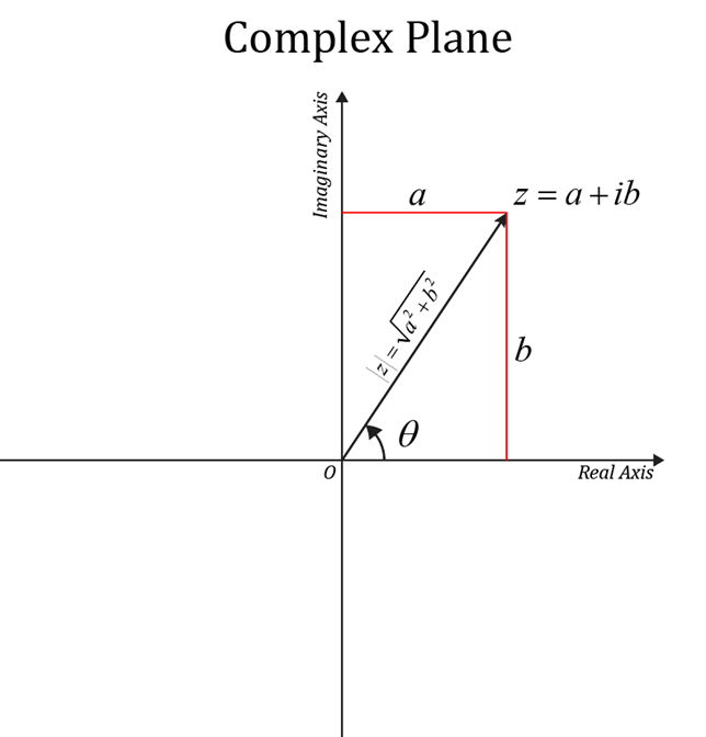
- complex analysis
- tensor analysis
- group theory
These tools allow precise modeling of physical systems.
11. Symmetry in Physics
Symmetry plays a crucial role in physical laws.
Symmetry principles help simplify equations and reveal conservation laws.
Example:
Rotational symmetry leads to conservation of angular momentum.
Group theory is often used to analyze symmetries.
12. Conservation Laws
Physical systems often follow conservation laws.
Examples include:
- conservation of energy
- conservation of momentum
- conservation of charge
Mathematical physics studies how these laws arise from symmetries.
13. Wave Phenomena
Waves appear in many areas of physics.
Examples:
- sound waves
- light waves
- water waves
- quantum waves
Mathematical physics uses wave equations and Fourier analysis to study wave behavior.
14. Field Theory
Field theory studies physical quantities distributed in space.
Examples:
- electromagnetic fields
- gravitational fields
- quantum fields
Fields are represented mathematically as functions of space and time.
15. Mathematical Physics in Engineering
Engineering applications include:
- electrical circuits
- signal processing
- mechanical systems
- structural analysis
Mathematical models help engineers design and optimize systems.
16. Computational Methods
Modern mathematical physics often relies on computational techniques.
Examples include:
- numerical simulations
- finite element methods
- computational fluid dynamics
These methods solve equations that cannot be solved analytically.
17. Mathematical Physics in Cosmology
Cosmology studies the structure and evolution of the universe.
Mathematical physics helps explain:
- cosmic expansion
- dark matter
- dark energy
- black holes
Einstein’s field equations describe gravitational effects on a cosmic scale.
18. Mathematical Physics in Quantum Field Theory
Quantum field theory combines quantum mechanics and relativity.
It describes fundamental particle interactions.
Mathematical tools used include:
- operator theory
- path integrals
- symmetry groups
19. Importance of Mathematical Physics
Mathematical physics provides a deep understanding of the laws governing nature.
It allows scientists to:
- develop physical theories
- predict experimental results
- unify different branches of physics
Many modern technologies rely on theories developed in mathematical physics.
20. Modern Developments
Current research areas include:
- string theory
- quantum gravity
- condensed matter physics
- topological quantum computing
These fields explore fundamental questions about the universe.
Conclusion
Mathematical physics is a powerful interdisciplinary field that combines mathematical rigor with physical insight to describe and understand the natural world. By translating physical phenomena into mathematical equations and models, scientists can analyze complex systems, predict outcomes, and develop new technologies.
From classical mechanics and electromagnetism to quantum mechanics and relativity, mathematical physics provides the theoretical framework for modern science. Its reliance on advanced mathematical tools such as differential equations, linear algebra, and tensor analysis allows researchers to explore deep connections between mathematics and the fundamental laws of nature.
As scientific knowledge continues to advance, mathematical physics remains a cornerstone of theoretical research, helping scientists uncover the underlying structure of the universe and guiding technological innovation.