Category Archives: Mathematics

Inequalities in Mathematics

Introduction to Inequalities

In mathematics, inequalities are mathematical statements that compare two expressions and show that one quantity is greater than, less than, greater than or equal to, or less than or equal to another quantity. Unlike equations, which state that two expressions are equal, inequalities describe relationships where values are not necessarily equal but follow a certain order.

Inequalities are widely used in algebra, calculus, optimization, economics, engineering, statistics, and many scientific disciplines. They help represent real-world conditions where values are restricted within certain limits rather than fixed to a single number.

For example, consider the statement:

[
x > 5
]

This inequality indicates that the variable (x) can take any value greater than 5. Unlike equations, which typically have specific solutions, inequalities usually have a range of possible solutions.

Inequalities are particularly useful when modeling practical situations such as budget constraints, physical limits, safety ranges, or performance thresholds.

Definition of Inequality

An inequality is a mathematical relation that compares two expressions and indicates that one is larger or smaller than the other.

General form:

[
a < b
]

[
a > b
]

where (a) and (b) are expressions.

Instead of equality, inequalities use special symbols to show the relationship between values.

Inequality Symbols

The following symbols are commonly used in mathematics to represent inequalities.

Less Than

Symbol:

[
<
]

Example:

[
3 < 7
]

Meaning: 3 is less than 7.

Greater Than

Symbol:

[

]

Example:

[
9 > 4
]

Meaning: 9 is greater than 4.

Less Than or Equal To

Symbol:

[
\le
]

Example:

[
x \le 10
]

Meaning: (x) can be less than or equal to 10.

Greater Than or Equal To

Symbol:

[
\ge
]

Example:

[
x \ge 2
]

Meaning: (x) can be greater than or equal to 2.

Not Equal To

Symbol:

[
\neq
]

Example:

[
x \neq 3
]

Meaning: (x) cannot be equal to 3.

Types of Inequalities

Inequalities can be categorized into several types depending on their structure.

Linear Inequalities

A linear inequality contains variables raised only to the first power.

Example:

[
2x + 3 > 7
]

Solving:

[
2x > 4
]

[
x > 2
]

Linear inequalities produce solution intervals rather than single values.

Quadratic Inequalities

A quadratic inequality contains variables raised to the power of 2.

Example:

[
x^2 – 5x + 6 > 0
]

First factor:

[
(x-2)(x-3) > 0
]

Then determine intervals where the expression is positive.

Quadratic inequalities typically produce multiple solution ranges.

Polynomial Inequalities

These involve higher degree polynomials.

Example:

[
x^3 – x > 0
]

Solve by factoring and testing intervals.

Rational Inequalities

A rational inequality contains fractions with variables.

Example:

[
\frac{x+2}{x-3} > 0
]

Solve by determining where numerator and denominator change signs.

Absolute Value Inequalities

These involve absolute value expressions.

Example:

[
|x-4| < 3
]

Meaning the distance between (x) and 4 is less than 3.

Solution:

[
1 < x < 7
]

Absolute value inequalities often produce compound inequalities.

Compound Inequalities

A compound inequality combines two inequalities together.

Example:

[
3 < x < 7
]

Meaning:

[
x > 3 \text{ AND } x < 7
]

Compound inequalities describe values within a specific interval.

Graphing Inequalities

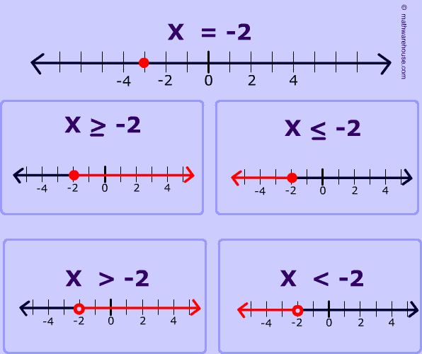
Inequalities can be represented graphically using number lines or coordinate planes.

Graphing on a Number Line

Example:

[
x > 3
]

Steps:

Draw number line.
Place open circle at 3.
Shade to the right.

Open circle means the endpoint is not included.

Example:

[
x \le 5
]

Steps:

Place closed circle at 5.
Shade to the left.

Closed circle means the endpoint is included.

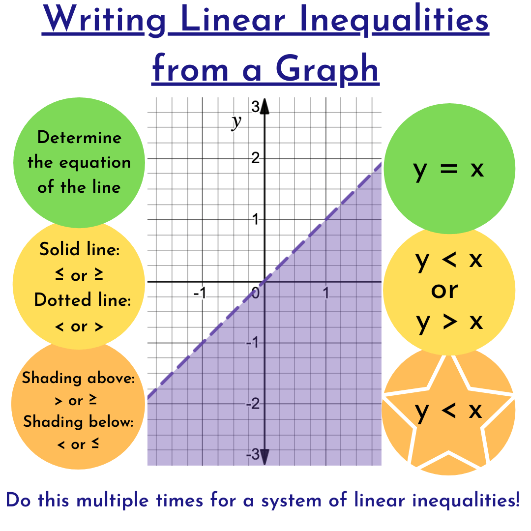
Graphing Linear Inequalities in Two Variables

Example:

[
y > 2x + 1
]

Steps:

Graph line (y = 2x + 1).
Use dashed line (since inequality is strict).
Shade region above the line.

If inequality is ≥ or ≤, use solid line.

Systems of Inequalities

A system of inequalities involves two or more inequalities solved together.

Example:

[
y > x
]

[
y < 2x + 3
]

Solution is the region that satisfies both conditions simultaneously.

This is shown as the overlapping shaded region on a graph.

Properties of Inequalities

Inequalities follow several algebraic rules.

Addition Property

Adding the same number to both sides keeps inequality true.

Example:

[
x > 3
]

Add 5:

[
x + 5 > 8
]

Subtraction Property

Subtracting same number maintains inequality.

Example:

[
x + 4 < 9
]

Subtract 4:

[
x < 5
]

Multiplication Property

Multiplying both sides by positive number keeps inequality same.

Example:

[
x > 2
]

Multiply by 3:

[
3x > 6
]

Negative Multiplication Rule

Multiplying by a negative number reverses the inequality.

Example:

[
x > 2
]

Multiply by -1:

[
-x < -2
]

Division Property

Dividing both sides by positive number keeps inequality same.

Dividing by negative reverses it.

Interval Notation

Solutions to inequalities are often expressed using interval notation.

Examples:

[
x > 3
]

Interval:

[
(3, \infty)
]

Example:

[
2 \le x < 6
]

Interval:

[
[2, 6)
]

Symbols meaning:

( ) = endpoint excluded
[ ] = endpoint included

Solving Inequalities

Solving inequalities follows similar steps as solving equations.

Example:

[
3x + 4 > 10
]

Step 1:

[
3x > 6
]

Step 2:

[
x > 2
]

Solving Quadratic Inequalities

Example:

[
x^2 – 5x + 6 < 0
]

Step 1: Factor

[
(x-2)(x-3) < 0
]

Step 2: Determine intervals

Solution:

[
2 < x < 3
]

Solving Absolute Value Inequalities

Example:

[
|x-5| < 2
]

Rewrite as compound inequality:

[
-2 < x-5 < 2
]

Add 5:

[
3 < x < 7
]

Inequalities in Calculus

Inequalities are essential in calculus for:

Limits
Optimization
Bounding functions
Convergence analysis

Example:

[
|f(x)| \le g(x)
]

Used in comparison tests.

Important Inequalities in Mathematics

Many famous inequalities are fundamental in advanced mathematics.

Triangle Inequality

States:

[
|a + b| \le |a| + |b|
]

Used in:

geometry
vector analysis
complex numbers

Cauchy–Schwarz Inequality

Important in linear algebra.

[
(a_1b_1 + a_2b_2 + … + a_nb_n)^2 \le (a_1^2 + …)(b_1^2 + …)
]

Used in:

statistics
machine learning
physics

Arithmetic Mean – Geometric Mean Inequality (AM-GM)

[
\frac{a+b}{2} \ge \sqrt{ab}
]

Important in optimization problems.

Applications of Inequalities

Inequalities appear in many practical situations.

Economics

Used in:

cost constraints
profit maximization
budget limitations

Example:

[
cost \le budget
]

Engineering

Used to maintain safety conditions.

Example:

Stress must remain below maximum threshold.

Physics

Used to define ranges.

Example:

Speed must be less than escape velocity.

Computer Science

Used in:

algorithm complexity analysis
optimization
machine learning constraints

Statistics

Used in probability bounds such as:

Chebyshev inequality
Markov inequality

Optimization Problems

Inequalities define constraints in optimization.

Example:

Maximize profit:

[
P = 5x + 3y
]

Subject to:

[
x + y \le 10
]

[
x \ge 0
]

[
y \ge 0
]

Solution found using linear programming.

Inequalities in Geometry

Geometry uses inequalities extensively.

Example:

Triangle inequality:

Sum of any two sides must be greater than third side.

Inequalities in Number Theory

Number theory uses inequalities to analyze integer relationships.

Example:

Prime number bounds.

Historical Development

Inequalities have been studied since ancient mathematics.

Ancient Greek mathematicians used inequalities in geometric proofs.

Later developments in algebra introduced symbolic representation of inequalities.

In modern mathematics, inequalities are central in fields such as optimization theory and functional analysis.

Importance of Inequalities

Inequalities help:

Describe ranges instead of exact values
Model real-world constraints
Analyze function behavior
Optimize solutions

They form the backbone of many mathematical models.

Conclusion

Inequalities are an essential part of mathematics that describe relationships between quantities when exact equality is not required. From simple comparisons between numbers to complex systems that govern optimization problems and advanced theoretical mathematics, inequalities provide powerful tools for analyzing and understanding mathematical relationships.

Their applications span across science, engineering, economics, statistics, and computer science. Mastering inequalities enables mathematicians and scientists to define limits, evaluate constraints, and solve practical problems involving ranges of values.

Understanding inequalities not only strengthens algebraic skills but also builds a foundation for advanced mathematical topics such as calculus, optimization, and mathematical modeling.

Polynomials — A Complete Guide in Mathematics

Leave a reply

Introduction to Polynomials

In mathematics, polynomials are one of the most fundamental and widely used algebraic structures. They appear in algebra, calculus, number theory, engineering, economics, physics, computer science, and many other fields. A polynomial is an algebraic expression composed of variables, constants, and exponents combined using addition, subtraction, and multiplication.

Unlike many other mathematical expressions, polynomials do not include variables in denominators, negative exponents, fractional exponents, or radicals involving variables. Because of this restriction, polynomials are relatively easy to analyze and manipulate, making them essential building blocks in mathematics.

A simple example of a polynomial is:

[
3x^2 + 2x + 5
]

In this expression:

3x² is a term
2x is another term
5 is the constant term

Together they form a polynomial expression.

Polynomials are important because they can approximate complex functions, describe curves and surfaces, represent physical phenomena, and solve real-world problems.

Definition of Polynomial

A polynomial is an expression of the form:

[
a_n x^n + a_{n-1} x^{n-1} + \dots + a_2 x^2 + a_1 x + a_0
]

Where:

x = variable
a₀, a₁, a₂ … aₙ = constants called coefficients
n = non-negative integer (degree of polynomial)

Example:

[
4x^3 + 2x^2 – 7x + 9
]

Here:

Degree = 3
Coefficients = 4, 2, -7
Constant = 9

Components of a Polynomial

A polynomial consists of several important parts.

1. Terms

A term is a single part of a polynomial separated by addition or subtraction.

Example:

[
5x^3 + 2x^2 – 4x + 7
]

Terms are:

5x³
2x²
-4x
7

2. Coefficient

The coefficient is the numerical factor multiplied by the variable.

Example:

In 6x², the coefficient is 6.

3. Constant

The constant term has no variable.

Example:

[
4x^3 + 5x – 8
]

Constant = -8

4. Degree

The degree of a polynomial is the highest exponent of the variable.

Example:

[
7x^4 + 3x^2 + x + 1
]

Degree = 4

Types of Polynomials Based on Number of Terms

Polynomials can be classified based on how many terms they contain.

Monomial

A polynomial with one term.

Examples:

[
5x^2
]

[
7y
]

[
3
]

Binomial

A polynomial with two terms.

Examples:

[
x + 5
]

[
3x^2 – 7
]

Trinomial

A polynomial with three terms.

Examples:

[
x^2 + 3x + 5
]

[
2x^2 – x + 7
]

Polynomial (General)

A polynomial with more than three terms.

Example:

[
x^4 + 2x^3 + 3x^2 + x + 6
]

Types of Polynomials Based on Degree

Polynomials are also classified by degree.

Constant Polynomial

Degree = 0

Example:

[
7
]

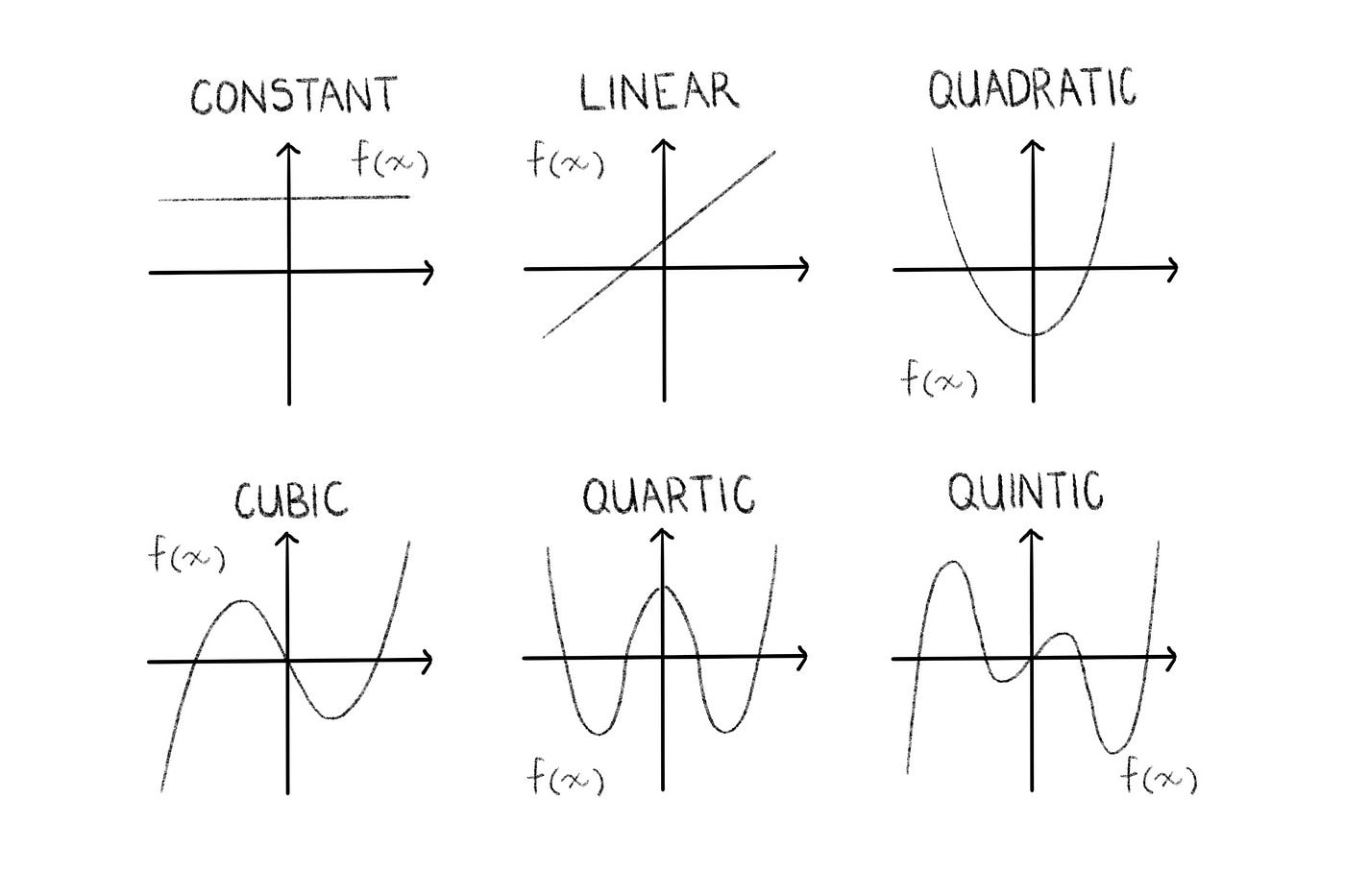
Linear Polynomial

Degree = 1

Example:

[
2x + 3
]

Graph of a linear polynomial is a straight line.

Quadratic Polynomial

Degree = 2

Example:

[
x^2 + 3x + 2
]

Graph is a parabola.

Cubic Polynomial

Degree = 3

Example:

[
x^3 + 2x^2 – x + 5
]

Graph can have up to two turning points.

Quartic Polynomial

Degree = 4

Example:

[
x^4 + 2x^2 + 1
]

Graph can have three turning points.

Quintic Polynomial

Degree = 5

Example:

[
x^5 + 2x^3 + x + 7
]

Higher degree polynomials have more complex curves.

Polynomial Functions

A polynomial function is a function defined by a polynomial expression.

Example:

[
f(x) = 2x^3 – x + 5
]

This function maps values of x to values of f(x).

Polynomial functions are continuous and smooth.

Properties:

No sharp corners
No breaks
No vertical asymptotes

Operations on Polynomials

Polynomials can be manipulated using various algebraic operations.

Addition of Polynomials

Add like terms.

Example:

[
(3x^2 + 2x + 5) + (2x^2 + 4x + 1)
]

Result:

[
5x^2 + 6x + 6
]

Subtraction of Polynomials

Example:

[
(5x^2 + 4x + 3) – (2x^2 + x + 1)
]

Result:

[
3x^2 + 3x + 2
]

Multiplication of Polynomials

Example:

[
(x + 2)(x + 3)
]

Using distributive property:

[
x^2 + 5x + 6
]

Division of Polynomials

Division methods include:

Long division
Synthetic division

Example:

[
(x^2 + 5x + 6) ÷ (x + 2)
]

Result:

[
x + 3
]

Factoring Polynomials

Factoring means writing a polynomial as a product of simpler polynomials.

Example:

[
x^2 + 5x + 6
]

Factor:

[
(x + 2)(x + 3)
]

Common factoring methods:

Greatest Common Factor (GCF)
Factoring trinomials
Difference of squares
Sum and difference of cubes
Grouping

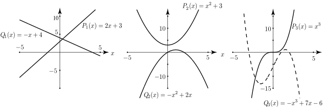
Polynomial Graphs

The graph of a polynomial shows how the function behaves.

Key features:

Intercepts

x-intercept → where graph crosses x-axis
y-intercept → where graph crosses y-axis

End Behavior

End behavior depends on:

Degree
Leading coefficient

Example:

If degree is even and coefficient positive:

Graph opens upwards on both sides.

Turning Points

A polynomial of degree n can have at most:

[
n-1
]

turning points.

Polynomial Roots and Zeros

A root or zero of a polynomial is the value of x where:

[
f(x) = 0
]

Example:

[
x^2 – 5x + 6 = 0
]

Factor:

[
(x-2)(x-3)=0
]

Roots:

[
x = 2, 3
]

Fundamental Theorem of Algebra

The Fundamental Theorem of Algebra states:

Every polynomial equation of degree n has exactly n complex roots (counting multiplicity).

Example:

A cubic polynomial always has 3 roots.

Polynomial Theorems

Important theorems related to polynomials include:

Remainder Theorem

If polynomial f(x) is divided by (x − a), remainder is:

[
f(a)
]

Factor Theorem

If:

[
f(a) = 0
]

then (x − a) is a factor.

Applications of Polynomials

Polynomials are widely used in real-world applications.

Physics

Used to describe motion, trajectories, and physical systems.

Example:

Projectile motion equations.

Engineering

Used in:

Structural design
Signal processing
Control systems

Economics

Used to model:

Cost functions
Revenue functions
Profit functions

Computer Graphics

Curves in animation and design often use polynomial interpolation.

Example:

Bezier curves.

Statistics

Regression models use polynomial equations to fit data.

Polynomial Interpolation

Polynomial interpolation is used to find a polynomial that passes through given data points.

Example:

Given points:

(1,2), (2,3), (3,5)

A polynomial can be created that fits these points exactly.

Methods include:

Lagrange interpolation
Newton interpolation

Special Polynomials

Several special polynomials are important in mathematics.

Chebyshev Polynomials

Used in approximation theory.

Legendre Polynomials

Used in physics, especially in solving differential equations.

Hermite Polynomials

Used in probability theory and quantum mechanics.

Taylor Polynomials

Used in calculus to approximate functions.

Example:

[
e^x \approx 1 + x + x^2/2 + x^3/6
]

Multivariable Polynomials

Polynomials can have more than one variable.

Example:

[
3x^2y + 2xy^2 + 5
]

Variables:

x and y.

These are used in:

algebraic geometry
optimization
physics

Polynomial Rings

In abstract algebra, polynomials form a ring.

Example:

R[x]

This means polynomials with coefficients in ring R.

Polynomial rings are fundamental in:

algebra
coding theory
cryptography

Polynomial Approximation

Many complicated functions can be approximated using polynomials.

Example:

[
sin(x)
]

can be approximated using Taylor polynomial.

This concept is heavily used in:

numerical analysis
machine learning
scientific computing

Advantages of Polynomials

Polynomials are extremely useful because they:

Are easy to compute
Are continuous and smooth
Can approximate many functions
Are simple to differentiate and integrate

Limitations of Polynomials

Polynomials cannot represent:

Vertical asymptotes
Discontinuous functions
Exponential growth perfectly
Periodic behavior accurately over large intervals

Historical Development of Polynomials

The concept of polynomials has existed for thousands of years.

Ancient Civilizations

Babylonians solved quadratic equations around 2000 BCE.

Greek Mathematics

Greek mathematicians studied geometric interpretations of algebraic equations.

Islamic Golden Age

Persian mathematician Al-Khwarizmi developed systematic algebraic methods.

Renaissance Period

Italian mathematicians discovered formulas for solving cubic and quartic equations.

Modern Mathematics

Polynomials became central in algebra and calculus development.

Polynomials in Modern Technology

Polynomials are used in modern technologies including:

Computer graphics
Cryptography
Signal processing
Machine learning algorithms
Data fitting
Robotics motion planning

Conclusion

Polynomials are among the most important structures in mathematics. Their simplicity, flexibility, and powerful properties make them essential tools for both theoretical mathematics and practical applications.

From basic algebra taught in schools to advanced scientific research, polynomials play a crucial role in understanding patterns, solving equations, modeling real-world systems, and building modern technology.

Their ability to approximate complex functions, describe curves and shapes, and solve practical problems ensures that polynomials remain a central topic in mathematics and science.

Quadratic Equations in Mathematics

Leave a reply

Tags:

Quadratic Equations in Mathematics

Quadratic equations are a fundamental concept in algebra and play an important role in many areas of mathematics, science, engineering, economics, and computer science. A quadratic equation is a polynomial equation of degree two, meaning the highest power of the variable is two.

Quadratic equations appear in many real-world problems involving motion, geometry, optimization, and physics. They describe relationships where variables change in a non-linear way, producing a characteristic curved graph called a parabola.

For example:

x² − 5x + 6 = 0

This equation contains the squared variable x², which makes it quadratic.

Quadratic equations are studied extensively because they provide insight into how mathematical relationships behave when variables are squared. They also serve as the foundation for many advanced mathematical topics, including calculus, mathematical modeling, and differential equations.

1. Definition of a Quadratic Equation

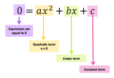
A quadratic equation is an equation of the form:

ax² + bx + c = 0

Where:

a, b, and c are constants
x is the variable
a ≠ 0

Example:

2x² + 3x − 5 = 0

In this equation:

a = 2
b = 3
c = −5

The term x² indicates that the equation is quadratic.

2. Components of a Quadratic Equation

Quadratic equations contain several important components.

Variable

The unknown quantity represented by a letter.

Example:

x in the equation:

x² + 4x + 4 = 0

Coefficients

Coefficients are numerical values multiplying the variable terms.

Example:

In the equation:

3x² + 5x + 1 = 0

3 and 5 are coefficients.

Constant Term

The constant is the number without a variable.

Example:

In the equation:

x² + 6x + 9 = 0

The constant term is 9.

Quadratic Term

The term containing the squared variable.

Example:

4x²

3. Standard Form of Quadratic Equation

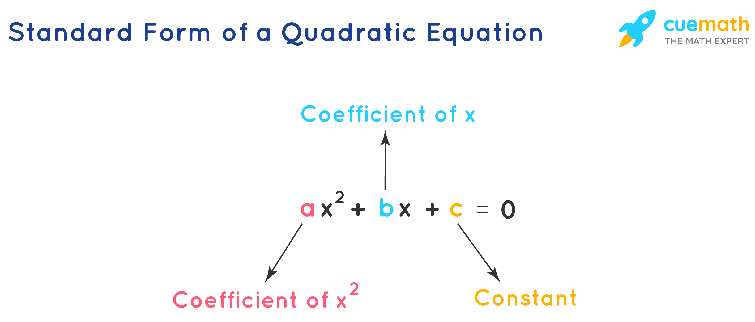
The general form is:

ax² + bx + c = 0

Where:

a determines the shape of the parabola
b influences the position
c determines the y-intercept

Example:

x² − 7x + 10 = 0

This equation follows the standard form.

4. Graph of Quadratic Equations

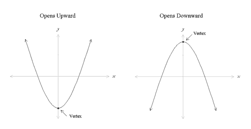
The graph of a quadratic equation is called a parabola.

Characteristics of a parabola include:

a curved shape
symmetry
a vertex

Vertex

The vertex is the highest or lowest point of the parabola.

If the parabola opens upward, the vertex is the minimum point.

If it opens downward, the vertex is the maximum point.

Axis of Symmetry

The vertical line that divides the parabola into two identical halves.

Equation:

x = −b / 2a

Direction of Opening

If:

a > 0 → parabola opens upward

a < 0 → parabola opens downward

5. Methods of Solving Quadratic Equations

There are several methods to solve quadratic equations.

5.1 Factoring Method

Factoring rewrites the quadratic expression as a product of two binomials.

Example:

x² + 5x + 6 = 0

Factor:

(x + 2)(x + 3) = 0

Solutions:

x = −2
x = −3

5.2 Completing the Square

This method transforms a quadratic equation into a perfect square.

Example:

x² + 6x + 5 = 0

Step 1:

x² + 6x = −5

Step 2:

Add 9 to both sides

(x + 3)² = 4

Step 3:

Take square root

x + 3 = ±2

Solutions:

x = −1 or x = −5

5.3 Quadratic Formula

The quadratic formula solves any quadratic equation.

Formula:

x = (−b ± √(b² − 4ac)) / 2a

Example:

x² − 5x + 6 = 0

Substitute values:

a = 1
b = −5
c = 6

Solutions:

x = 2
x = 3

6. The Discriminant

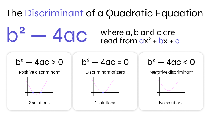
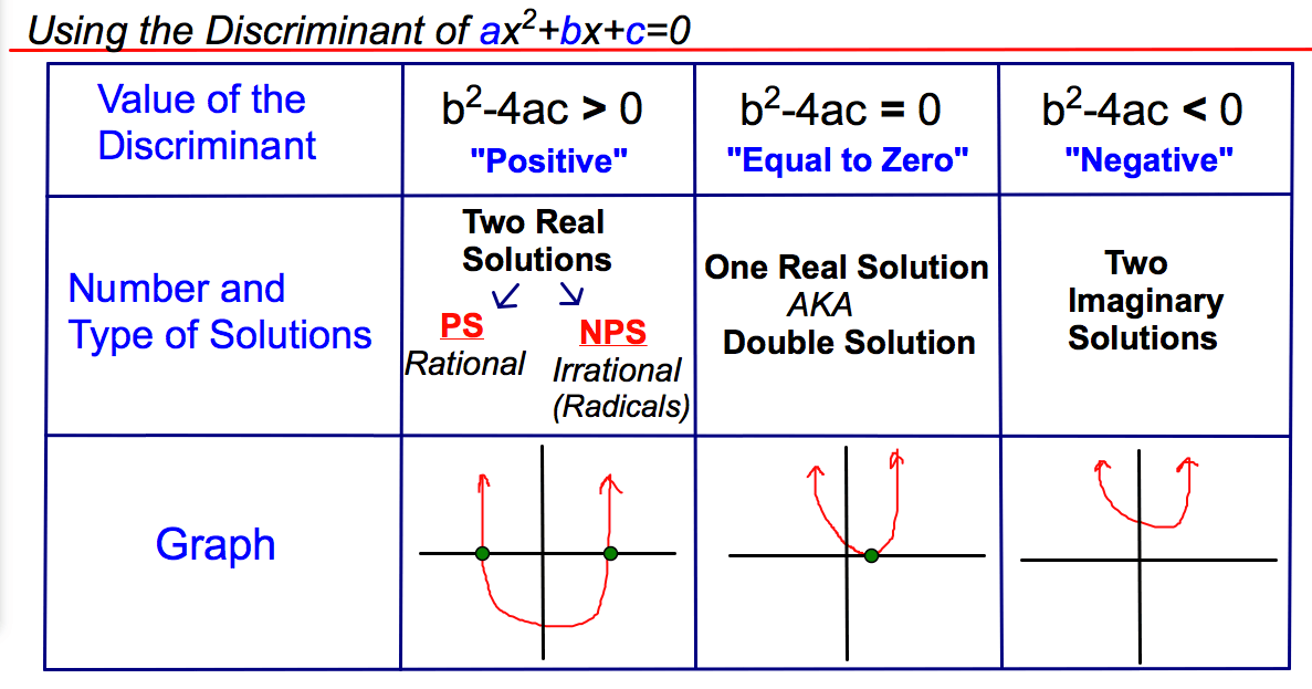
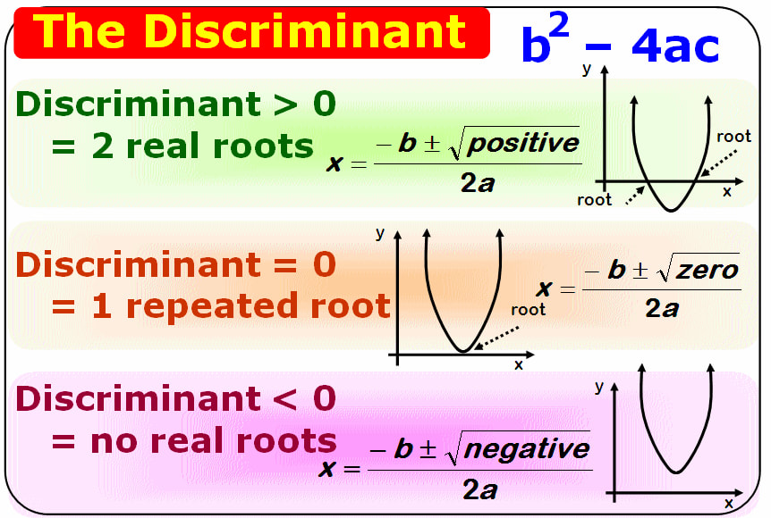
The discriminant determines the nature of the solutions.

Discriminant formula:

D = b² − 4ac

Cases

D > 0

Two real and distinct roots.

D = 0

One real repeated root.

D < 0

Two complex roots.

7. Roots of Quadratic Equations

Roots are values of x that satisfy the equation.

Example:

x² − 9 = 0

Factor:

(x − 3)(x + 3) = 0

Roots:

3 and −3

These roots represent the points where the graph crosses the x-axis.

8. Vertex Form of Quadratic Equation

Another form is:

y = a(x − h)² + k

Where:

(h, k) represents the vertex.

Example:

y = (x − 2)² + 3

Vertex:

(2, 3)

9. Quadratic Functions

A quadratic function describes a relationship between variables.

Example:

f(x) = x² + 2x + 1

The output depends on the input value of x.

Quadratic functions model many real-world processes.

10. Applications of Quadratic Equations

Quadratic equations appear in many real-world situations.

Physics

Projectile motion follows a quadratic path.

Example:

Height of a thrown object.

Engineering

Quadratic equations help calculate structural curves.

Economics

Profit and cost functions often form quadratic relationships.

Architecture

Parabolic arches use quadratic shapes.

11. Quadratic Equations in Geometry

Quadratic equations appear in geometric problems.

Example:

Area formulas.

Example:

Area of square:

A = x²

12. Maximum and Minimum Values

Quadratic functions can have maximum or minimum values.

Example:

y = x² − 4x + 3

Vertex gives minimum value.

These concepts are important in optimization problems.

13. Quadratic Inequalities

Quadratic inequalities involve expressions like:

x² − 5x + 6 > 0

Solutions represent ranges of values.

Graphical methods help identify solution intervals.

14. Quadratic Equations in Coordinate Geometry

Quadratic equations describe curves in coordinate geometry.

Example:

Parabolas

They are used to analyze geometric relationships.

15. Relationship Between Roots and Coefficients

For equation:

ax² + bx + c = 0

Sum of roots:

−b / a

Product of roots:

c / a

These relationships help analyze equations quickly.

16. Historical Development

Quadratic equations have been studied for thousands of years.

Ancient civilizations developed methods to solve quadratic problems in geometry and commerce.

Mathematicians later formalized algebraic methods that led to the modern quadratic formula.

17. Quadratic Equations in Advanced Mathematics

Quadratic equations lead to many advanced topics including:

polynomial theory
calculus
complex numbers
mathematical modeling

These topics expand the study of quadratic relationships.

18. Importance of Quadratic Equations

Quadratic equations are important because they:

describe curved relationships
model real-world phenomena
help solve optimization problems
form the basis of many mathematical theories

They are essential in mathematics education.

19. Quadratic Equations in Computer Science

Quadratic equations appear in:

graphics rendering
optimization algorithms
physics simulations
machine learning models

Computational methods often solve quadratic equations efficiently.

20. Summary

Quadratic equations are polynomial equations of degree two that play a crucial role in algebra and many scientific disciplines. Their characteristic parabolic graphs make them useful for modeling real-world phenomena involving curved motion and optimization.

Understanding quadratic equations involves learning their structure, graphical representation, solving methods, and applications. Techniques such as factoring, completing the square, and using the quadratic formula allow mathematicians to find solutions efficiently.

Because of their wide range of applications in physics, engineering, economics, and computer science, quadratic equations remain one of the most important topics in mathematics.

Linear Equations in Mathematics

Leave a reply

Tags:

Linear Equations in Mathematics

Linear equations are one of the most fundamental topics in algebra and mathematics. They represent relationships between variables that form straight-line graphs when plotted on a coordinate plane. Linear equations are widely used in mathematics, physics, economics, engineering, computer science, and many other scientific disciplines.

A linear equation is an equation in which the highest power of the variable is one. This means the variables are not squared, cubed, or raised to higher powers. Linear equations describe relationships that change at a constant rate.

For example:

2x + 3 = 7

This equation contains a variable x, constants 2, 3, and 7, and the equation shows a relationship that can be solved to find the value of x.

Linear equations are essential because they form the basis for understanding more advanced mathematical concepts such as systems of equations, matrices, calculus, and mathematical modeling.

1. Definition of a Linear Equation

A linear equation is an algebraic equation in which each variable has an exponent of one, and the equation forms a straight line when graphed.

General form:

ax + b = 0

Where:

a and b are constants
x is a variable

Example:

3x + 5 = 11

Here:

3 is the coefficient
5 is the constant term
x is the variable

Linear equations are called “linear” because they produce linear graphs (straight lines).

2. Components of a Linear Equation

Linear equations contain several key components.

Variables

Variables represent unknown values.

Example:

x, y, z

Example equation:

2x + 4 = 10

Here x is the variable.

Constants

Constants are fixed numbers.

Example:

In the equation:

3x + 7 = 16

The numbers 7 and 16 are constants.

Coefficients

A coefficient is a number multiplied by a variable.

Example:

Here 5 is the coefficient.

Terms

Terms are parts of an equation separated by addition or subtraction.

Example:

4x + 6

Terms:

4x and 6

3. Types of Linear Equations

Linear equations can appear in several different forms.

Linear Equation in One Variable

These equations contain only one variable.

Example:

5x + 3 = 13

Solution:

5x = 10

x = 2

Linear Equation in Two Variables

These equations contain two variables.

Example:

2x + y = 6

Solutions include pairs of numbers that satisfy the equation.

Example:

x = 2, y = 2

Linear Equation in Three Variables

Example:

x + y + z = 6

These equations are used in advanced algebra and linear systems.

4. Standard Form of Linear Equation

The standard form of a linear equation in two variables is:

Ax + By + C = 0

Where:

A, B, and C are constants
A and B are not both zero

Example:

2x + 3y − 6 = 0

This form is useful in coordinate geometry.

5. Slope-Intercept Form

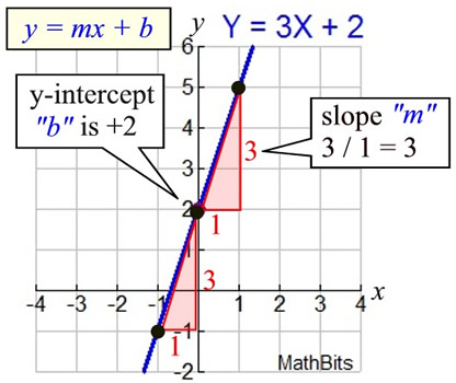
Another important form is:

y = mx + b

Where:

m is the slope
b is the y-intercept

Example:

y = 2x + 3

Slope = 2
Intercept = 3

This means the line crosses the y-axis at 3.

6. Graph of Linear Equations

A linear equation in two variables represents a straight line on a coordinate plane.

Steps to graph a linear equation:

Convert equation into slope-intercept form.
Identify slope and intercept.
Plot the intercept.
Use the slope to find additional points.
Draw a straight line through the points.

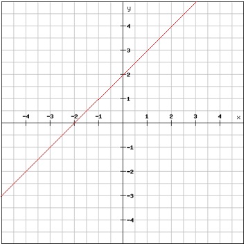
Example:

y = x + 2

Points:

(0,2)

(1,3)

(2,4)

These points form a straight line.

7. Solving Linear Equations

Solving a linear equation means finding the value of the variable.

Example 1

3x + 5 = 11

Step 1:

Subtract 5

3x = 6

Step 2:

Divide by 3

x = 2

Example 2

5x − 4 = 16

Add 4:

5x = 20

Divide by 5:

x = 4

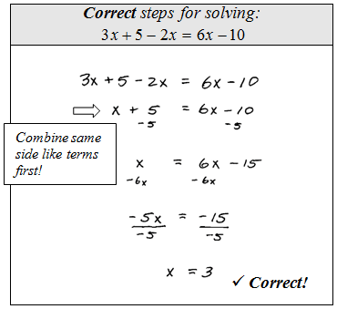
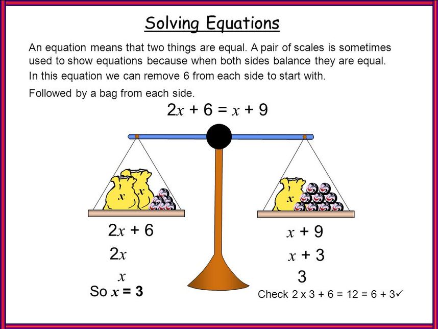
8. Linear Equations with Variables on Both Sides

Example:

2x + 5 = x + 9

Step 1:

Subtract x from both sides

x + 5 = 9

Step 2:

Subtract 5

x = 4

9. Systems of Linear Equations

A system of linear equations contains two or more equations with the same variables.

Example:

x + y = 5
x − y = 1

The solution is the point where both equations are satisfied.

10. Methods for Solving Systems

Substitution Method

Solve one equation for a variable and substitute into the other.

Example:

x = 5 − y

Substitute into the second equation.

Elimination Method

Add or subtract equations to eliminate a variable.

Example:

x + y = 5
x − y = 1

Add equations:

2x = 6

x = 3

Substitute:

y = 2

Graphical Method

Plot both equations on a graph.

The intersection point is the solution.

11. Special Cases of Linear Systems

Systems may have:

One Solution

Lines intersect at one point.

Infinite Solutions

Lines overlap completely.

No Solution

Lines are parallel.

12. Linear Equations in Real-Life Applications

Linear equations appear in many practical situations.

Economics

Profit equations:

Profit = Revenue − Cost

Physics

Motion equation:

distance = speed × time

Business

Cost calculations:

Total cost = fixed cost + variable cost

Engineering

Linear models describe relationships between variables.

13. Linear Functions

A linear function describes a relationship between variables.

Example:

f(x) = 3x + 2

This function produces a straight line graph.

Linear functions describe constant rates of change.

14. Linear Equations in Coordinate Geometry

Linear equations represent lines on a coordinate plane.

Key concepts include:

slope
intercepts
parallel lines
perpendicular lines

Parallel Lines

Parallel lines have the same slope.

Example:

y = 2x + 3
y = 2x − 4

Perpendicular Lines

Perpendicular lines have slopes that are negative reciprocals.

Example:

Slope = 2

Perpendicular slope = −1/2

15. Linear Equations in Matrices

In higher mathematics, systems of linear equations can be represented using matrices.

Example:

AX = B

Matrix methods help solve large systems efficiently.

16. Importance of Linear Equations

Linear equations are essential because they:

describe relationships between variables
model real-world problems
provide a foundation for algebra

They are used extensively in science and technology.

17. Linear Equations in Computer Science

In computing, linear equations appear in:

machine learning
optimization algorithms
graphics transformations

Many algorithms rely on solving systems of linear equations.

18. Historical Development of Linear Algebra

The study of linear equations dates back to ancient civilizations.

Chinese mathematicians used methods similar to modern matrix techniques to solve systems of equations.

These ideas later developed into modern algebra and linear algebra.

19. Advanced Concepts Related to Linear Equations

Advanced topics include:

linear programming
vector spaces
matrix algebra
numerical methods

These topics extend the study of linear relationships.

20. Summary

Linear equations are fundamental mathematical expressions that represent relationships between variables where the highest exponent is one. These equations form straight lines when graphed and describe constant rates of change.

They are essential tools in algebra and are widely used in science, economics, engineering, and computer science. Understanding linear equations involves learning their forms, solving methods, graphical interpretation, and real-world applications.

Mastery of linear equations provides a strong foundation for advanced mathematics and problem-solving in many fields.

Algebraic Expressions in Mathematics

Leave a reply

Tags:

Algebraic Expressions in Mathematics

Algebraic expressions are one of the central concepts in algebra, a branch of mathematics that deals with symbols and the rules for manipulating those symbols. Algebraic expressions combine numbers, variables, and mathematical operations to represent mathematical relationships.

In simple terms, an algebraic expression is a mathematical phrase that may contain variables, constants, and arithmetic operations such as addition, subtraction, multiplication, and division. These expressions allow mathematicians and scientists to describe patterns, relationships, and general formulas.

For example:

3x + 5

This expression contains a variable x, a constant 5, and a coefficient 3.

Algebraic expressions are used in various fields such as physics, engineering, economics, and computer science to represent unknown values and perform calculations.

Understanding algebraic expressions is essential for learning more advanced mathematical topics like equations, functions, calculus, and mathematical modeling.

1. What is an Algebraic Expression?

An algebraic expression is a mathematical expression formed using:

numbers
variables
arithmetic operations

Example:

2x + 7

This expression represents a quantity that depends on the value of x.

Unlike equations, algebraic expressions do not contain an equals sign.

Example of an equation:

2x + 7 = 15

Example of an expression:

2x + 7

Expressions describe mathematical relationships but do not state equality.

2. Components of Algebraic Expressions

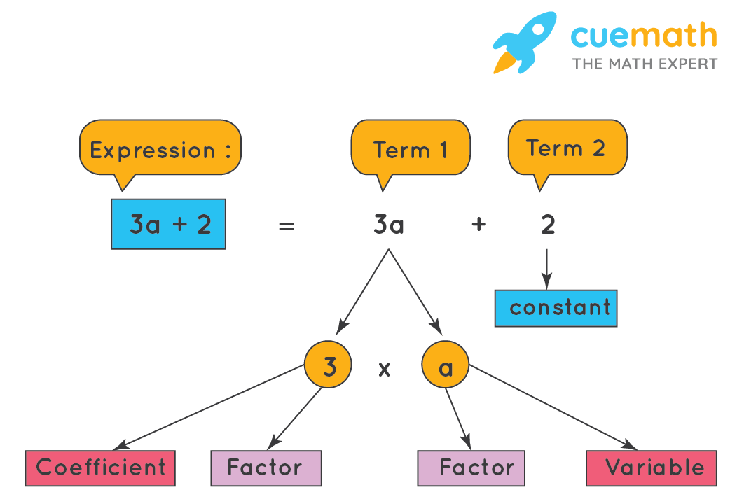
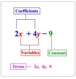
Algebraic expressions are made up of several key components.

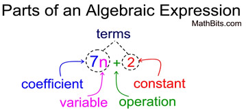
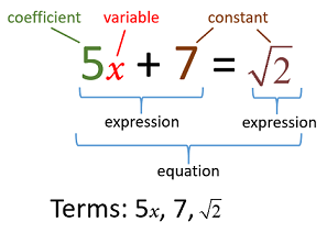
Variables

A variable is a symbol that represents an unknown value.

Common variables include:

x, y, z, a, b

Example:

5x + 2

Here x is the variable.

Variables allow expressions to represent many possible values.

Constants

A constant is a fixed numerical value.

Example:

In the expression:

3x + 8

The number 8 is a constant.

Constants do not change.

Coefficients

A coefficient is the numerical factor multiplied by a variable.

Example:

Here 4 is the coefficient.

Coefficients determine how much of a variable is present.

Terms

A term is a part of an expression separated by addition or subtraction.

Example:

5x + 3y − 2

Terms are:

5x, 3y, −2

3. Types of Algebraic Expressions

Expressions can be classified according to the number of terms.

Monomial

A monomial contains one term.

Example:

4y²

Binomial

A binomial contains two terms.

Example:

x + 5

3a − 2b

Trinomial

A trinomial contains three terms.

Example:

x² + 4x + 7

Polynomial

A polynomial contains one or more terms.

Example:

2x³ + 3x² − 5x + 6

Polynomials are widely studied in algebra.

4. Degree of an Algebraic Expression

The degree of an algebraic expression is determined by the highest exponent of the variable.

Example:

3x² + 2x + 5

The highest exponent is 2.

Degree = 2

Examples:

x³ + 2x² + 7 → degree 3
5x + 3 → degree 1

The degree helps classify polynomial expressions.

5. Algebraic Operations

Algebraic expressions can be manipulated using basic arithmetic operations.

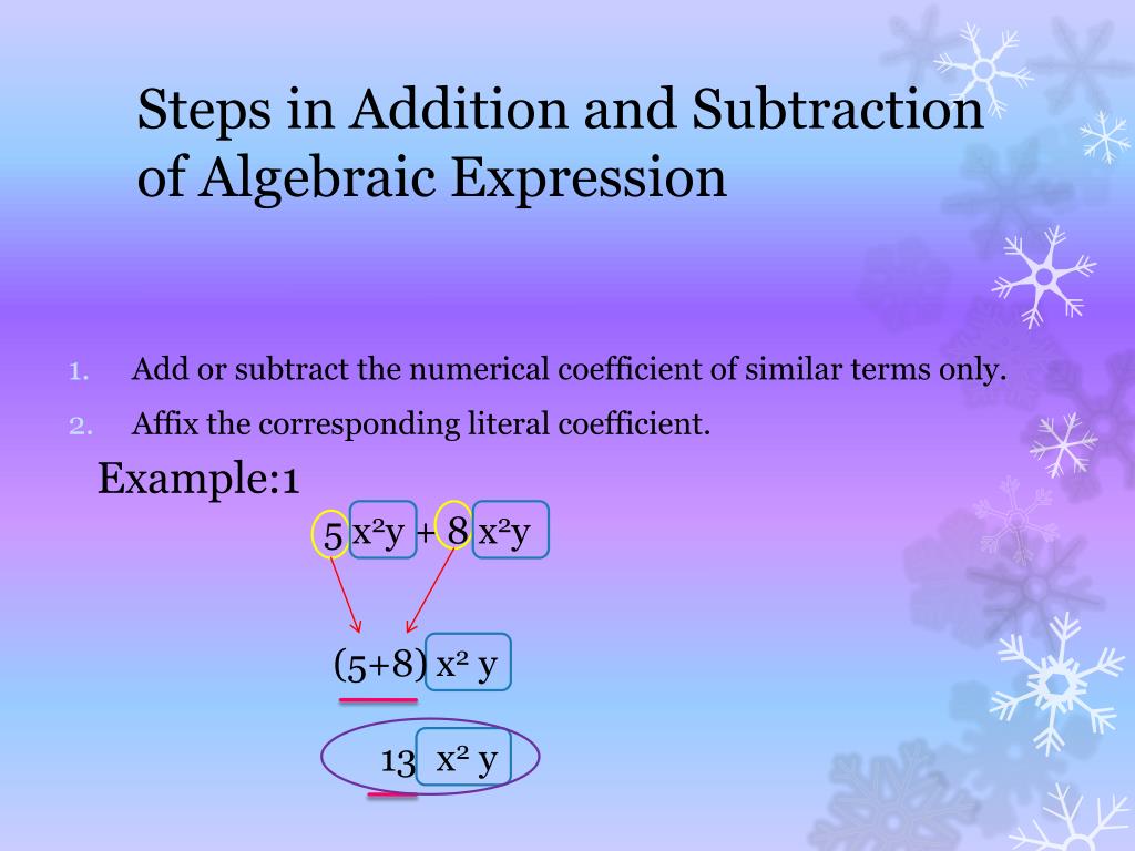
Addition of Algebraic Expressions

Add like terms together.

Example:

3x + 2x

Result:

Another example:

2x + 3 + 4x + 5

Combine like terms:

6x + 8

Subtraction of Algebraic Expressions

Example:

7x − 3x

Result:

Example:

(5x + 8) − (2x + 3)

Result:

3x + 5

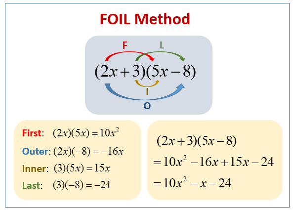
Multiplication of Algebraic Expressions

Example:

2x × 3x

Result:

6x²

Example:

(x + 2)(x + 3)

Using distributive property:

x² + 5x + 6

Division of Algebraic Expressions

Example:

6x² ÷ 3x

Result:

Division simplifies expressions.

6. Like Terms and Unlike Terms

Understanding like terms is essential for simplifying expressions.

Like Terms

Terms with the same variable and exponent.

Example:

3x and 5x

2y² and 7y²

These terms can be combined.

Example:

3x + 5x = 8x

Unlike Terms

Terms with different variables or exponents.

Example:

3x and 3y

2x² and 2x

These terms cannot be combined.

7. Simplifying Algebraic Expressions

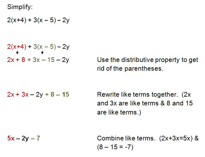
Simplifying means rewriting expressions in their simplest form.

Steps:

Identify like terms
Combine like terms
Arrange in standard form

Example:

3x + 2x + 4 − 1

Combine:

5x + 3

Example:

7y + 5 − 3y + 2

Result:

4y + 7

8. Evaluating Algebraic Expressions

Evaluating means finding the value of an expression when variables are replaced with numbers.

Example:

Expression:

2x + 5

If x = 3:

2(3) + 5

Result:

Example:

3a² − 4

If a = 2:

3(2²) − 4

Result:

9. Algebraic Expressions in Geometry

Algebraic expressions are used to represent geometric formulas.

Example:

Area of rectangle:

A = l × w

If length is:

x + 2

And width is:

Area expression:

x(x + 2)

Example:

Perimeter of square:

10. Algebraic Expressions and Real-Life Applications

Algebraic expressions are used in many practical situations.

Economics

Profit calculations:

Profit = revenue − cost

Physics

Distance formula:

d = vt

Engineering

Design calculations involve algebraic expressions.

Computer Science

Algorithms often use algebraic formulas.

11. Algebraic Identities

Important identities simplify algebraic expressions.

Examples include:

(a + b)² = a² + 2ab + b²

(a − b)² = a² − 2ab + b²

(a + b)(a − b) = a² − b²

These identities help expand or factor expressions.

12. Factorization

Factorization is the process of writing an expression as a product of factors.

Example:

x² + 5x + 6

Factors:

(x + 2)(x + 3)

Example:

x² − 9

Result:

(x − 3)(x + 3)

13. Importance of Algebraic Expressions

Algebraic expressions are important because they:

represent mathematical relationships
describe patterns
simplify calculations
help solve equations

They also form the basis of advanced mathematics.

14. Role in Higher Mathematics

Algebraic expressions are used in:

calculus
linear algebra
statistics
differential equations

They provide a symbolic way to represent mathematical models.

15. Algebraic Expressions and Functions

Functions often use algebraic expressions.

Example:

f(x) = 2x + 3

This function describes how outputs depend on inputs.

16. Historical Development of Algebra

The word algebra comes from the Arabic term “al-jabr.”

Early mathematicians developed symbolic methods to represent unknown quantities.

These ideas evolved into modern algebraic notation used today.

17. Algebraic Expressions in Scientific Models

Scientists use algebraic expressions to represent relationships between physical quantities.

Examples include:

motion equations
energy formulas
electrical circuits

These models help predict and analyze real-world phenomena.

18. Common Mistakes in Algebraic Expressions

Students often make mistakes such as:

combining unlike terms
forgetting negative signs
incorrect distribution

Example:

Incorrect:

3x + 2y = 5xy

Correct:

They cannot be combined.

19. Importance in Education

Learning algebraic expressions develops:

logical thinking
problem-solving skills
mathematical reasoning

These skills are valuable in many academic disciplines.

20. Summary

Algebraic expressions are mathematical expressions consisting of variables, constants, and operations. They provide a powerful way to represent mathematical relationships and unknown quantities.

Understanding algebraic expressions involves recognizing their components, performing operations, simplifying expressions, and applying them to real-world problems.

These expressions are fundamental to algebra and serve as the foundation for advanced mathematical concepts used in science, engineering, economics, and technology.

Basic Operations in Mathematics (Addition, Subtraction, Multiplication, Division)

Leave a reply

Tags:

Basic Operations in Mathematics (Addition, Subtraction, Multiplication, Division)

Basic operations form the foundation of mathematics and are essential for performing calculations in everyday life. The four primary arithmetic operations are addition, subtraction, multiplication, and division. These operations are used to combine numbers, find differences, determine repeated quantities, and distribute values.

These operations are fundamental to mathematics education and are the building blocks for more advanced topics such as algebra, geometry, statistics, and calculus. Every mathematical calculation, from simple counting to complex scientific computations, relies on these four operations.

The study of arithmetic operations dates back thousands of years, when early civilizations developed numerical systems to solve problems involving trade, agriculture, and construction. Over time, these operations evolved into the structured mathematical processes used today.

Understanding how these operations work and how they relate to one another is essential for developing strong mathematical reasoning and problem-solving skills.

1. Addition

Definition of Addition

Addition is the mathematical operation used to combine two or more numbers to obtain their total or sum.

The symbol used for addition is:

Example:

3 + 5 = 8

Here:

3 and 5 are called addends
8 is called the sum

Addition represents the concept of combining quantities.

Example:

If you have 3 apples and receive 2 more apples, the total number of apples becomes:

3 + 2 = 5

Understanding Addition

Addition can be visualized using objects or number lines.

Example:

Number line:

Start at 4 and move 3 steps forward.

4 + 3 = 7

Addition always moves toward larger numbers when dealing with positive numbers.

Properties of Addition

Addition follows several important mathematical properties.

Commutative Property

The order of numbers does not change the result.

a + b = b + a

Example:

3 + 7 = 7 + 3

Associative Property

The grouping of numbers does not change the result.

(a + b) + c = a + (b + c)

Example:

(2 + 3) + 4 = 2 + (3 + 4)

Identity Property

Adding zero does not change the number.

a + 0 = a

Example:

8 + 0 = 8

Addition with Larger Numbers

When adding multi-digit numbers, we align digits according to place value.

Example:

  345
+ 278
-----
  623

This method involves adding each column starting from the right.

2. Subtraction

Definition of Subtraction

Subtraction is the mathematical operation used to find the difference between two numbers.

The symbol used is:

−

Example:

9 − 4 = 5

Here:

9 is the minuend
4 is the subtrahend
5 is the difference

Subtraction represents removing or taking away quantities.

Understanding Subtraction

Example:

If you have 7 candies and give away 3 candies:

7 − 3 = 4

You now have 4 candies left.

Subtraction Using Number Line

Example:

8 − 3

Start at 8 and move 3 steps backward.

Result:

Borrowing in Subtraction

When subtracting multi-digit numbers, sometimes borrowing is required.

Example:

  402
- 178
-----
  224

Borrowing allows subtraction when the top digit is smaller than the bottom digit.

Properties of Subtraction

Subtraction does not satisfy commutative or associative properties.

Example:

5 − 3 ≠ 3 − 5

However, subtraction can be expressed as addition of negative numbers.

Example:

7 − 3 = 7 + (−3)

3. Multiplication

Definition of Multiplication

Multiplication is the operation of repeated addition.

The symbol used is:

Example:

4 × 3 = 12

This means:

4 + 4 + 4 = 12

Here:

4 and 3 are factors
12 is the product

Multiplication as Groups

Example:

3 groups of 5 apples.

3 × 5 = 15

Multiplication helps calculate repeated quantities efficiently.

Multiplication Table

The multiplication table helps perform multiplication quickly.

Example:

6 × 7 = 42

Learning multiplication tables is essential for arithmetic proficiency.

Properties of Multiplication

Commutative Property

a × b = b × a

Example:

5 × 4 = 4 × 5

Associative Property

(a × b) × c = a × (b × c)

Example:

(2 × 3) × 4 = 2 × (3 × 4)

Identity Property

a × 1 = a

Example:

9 × 1 = 9

Zero Property

a × 0 = 0

Example:

7 × 0 = 0

Multiplying Multi-Digit Numbers

Example:

  34
× 12
-----
  68
 340
-----
 408

This method multiplies digits step by step.

4. Division

Definition of Division

Division is the operation of splitting a quantity into equal parts.

The symbol used is:

Example:

12 ÷ 3 = 4

Here:

12 is the dividend
3 is the divisor
4 is the quotient

Division as Sharing

Example:

If 12 candies are shared among 3 children:

Each child gets:

4 candies

Division as Repeated Subtraction

Example:

12 ÷ 3

12 − 3 − 3 − 3 − 3

Four subtractions lead to zero.

Result:

Long Division

Example:

  84 ÷ 4

Step-by-step:

4 goes into 8 → 2
4 goes into 4 → 1

Result:

Division by Zero

Division by zero is undefined.

Example:

5 ÷ 0

This operation has no valid result in mathematics.

5. Relationships Between Operations

The four operations are interconnected.

Addition and subtraction are inverse operations.

Example:

8 − 3 = 5
5 + 3 = 8

Multiplication and division are also inverse operations.

Example:

4 × 5 = 20
20 ÷ 5 = 4

Understanding these relationships helps solve equations and check answers.

6. Order of Operations

When multiple operations appear in one expression, a specific order must be followed.

Common rule:

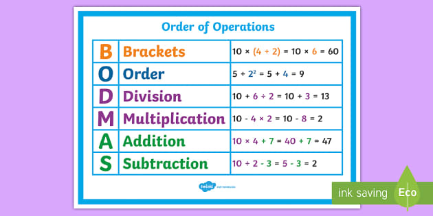
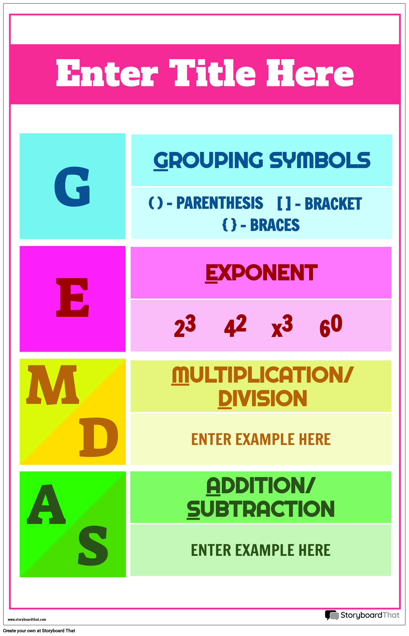
PEMDAS

Parentheses
Exponents
Multiplication
Division
Addition
Subtraction

Example:

3 + 5 × 2

First multiply:

5 × 2 = 10

Then add:

3 + 10 = 13

7. Applications in Daily Life

Basic operations are used in many everyday situations.

Shopping

Addition calculates total prices.

Subtraction determines change.

Example:

Total bill:

$10 + $5 + $3 = $18

Cooking

Recipes require multiplication and division.

Example:

Double a recipe:

2 cups → 4 cups

Travel

Multiplication calculates distance.

Example:

Speed × time.

Finance

Division calculates equal payments.

Example:

$100 divided among 4 people.

8. Basic Operations with Different Number Types

These operations apply to many number systems.

Examples include:

integers
fractions
decimals
rational numbers

Example with decimals:

2.5 + 1.3 = 3.8

Example with fractions:

1/2 + 1/4 = 3/4

9. Importance in Mathematics

Basic operations are the foundation of arithmetic.

They enable:

problem solving
logical reasoning
quantitative analysis

Without these operations, advanced mathematics would not exist.

10. Historical Development

Ancient civilizations developed arithmetic operations to solve practical problems.

Early mathematical systems appeared in:

ancient Egypt
Mesopotamia
India
Greece

Over centuries, these operations evolved into modern arithmetic methods.

11. Role in Modern Technology

Basic arithmetic operations are fundamental in computing.

Computers perform billions of calculations using these operations every second.

Applications include:

programming
algorithms
scientific computing
data analysis

12. Summary

Addition, subtraction, multiplication, and division are the four fundamental arithmetic operations in mathematics. They allow us to combine numbers, find differences, calculate repeated quantities, and divide quantities into equal parts.

These operations form the basis for mathematical reasoning and are used in nearly every aspect of daily life, including finance, science, engineering, and technology.

Understanding these basic operations is essential for learning advanced mathematical concepts and solving real-world problems effectively.

LCM and HCF in Mathematics

Leave a reply

Tags:

LCM and HCF in Mathematics

LCM (Least Common Multiple) and HCF (Highest Common Factor) are important concepts in arithmetic and number theory. These ideas help us understand how numbers relate to each other through multiples and factors. They are widely used in solving mathematical problems involving fractions, divisibility, scheduling, algebra, and real-life applications such as time cycles and resource distribution.

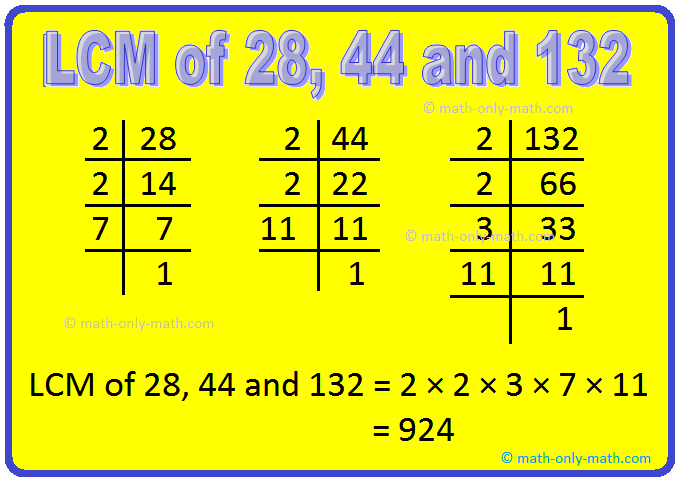
The Least Common Multiple (LCM) of two or more numbers is the smallest number that is a multiple of each of those numbers. The Highest Common Factor (HCF), also known as the Greatest Common Divisor (GCD), is the largest number that divides two or more numbers exactly.

Understanding LCM and HCF strengthens a student’s foundation in mathematics because these concepts appear frequently in arithmetic operations, algebraic expressions, and problem-solving scenarios.

1. Factors and Multiples

Before understanding LCM and HCF, it is important to understand factors and multiples.

Factors

A factor of a number is a number that divides another number exactly without leaving a remainder.

Example:

Factors of 12:

1, 2, 3, 4, 6, 12

Explanation:

12 ÷ 3 = 4
12 ÷ 6 = 2

Since the division leaves no remainder, these numbers are factors.

Multiples

A multiple of a number is obtained by multiplying that number by integers.

Example:

Multiples of 4:

4, 8, 12, 16, 20, 24, …

Multiples continue indefinitely because numbers can be multiplied by any integer.

2. Understanding HCF (Highest Common Factor)

Definition

The Highest Common Factor (HCF) of two or more numbers is the largest number that divides all of them exactly.

HCF is also called:

Greatest Common Divisor (GCD)
Greatest Common Factor (GCF)

Example:

Find the HCF of 12 and 18.

Factors of 12:

1, 2, 3, 4, 6, 12

Factors of 18:

1, 2, 3, 6, 9, 18

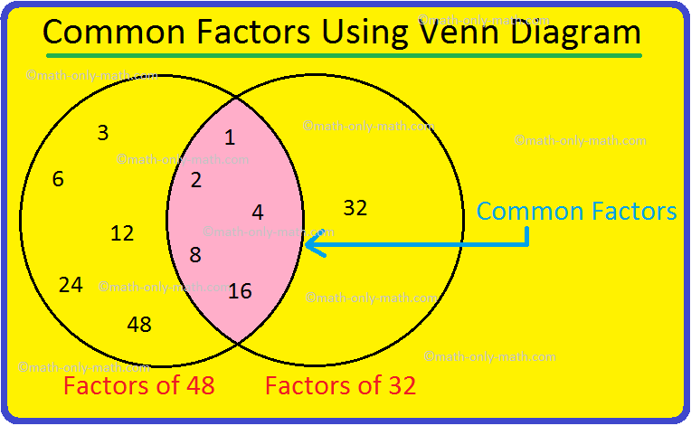
Common factors:

1, 2, 3, 6

Highest common factor:

Thus:

HCF(12,18) = 6

3. Methods to Find HCF

There are several methods for finding the HCF.

Factor Listing Method

List all factors of each number and find the greatest common factor.

Example:

Find HCF of 16 and 24.

Factors of 16:

1, 2, 4, 8, 16

Factors of 24:

1, 2, 3, 4, 6, 8, 12, 24

Common factors:

1, 2, 4, 8

HCF:

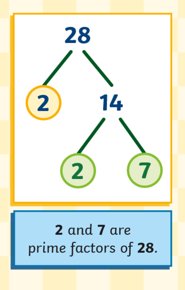
Prime Factorization Method

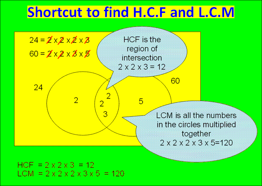
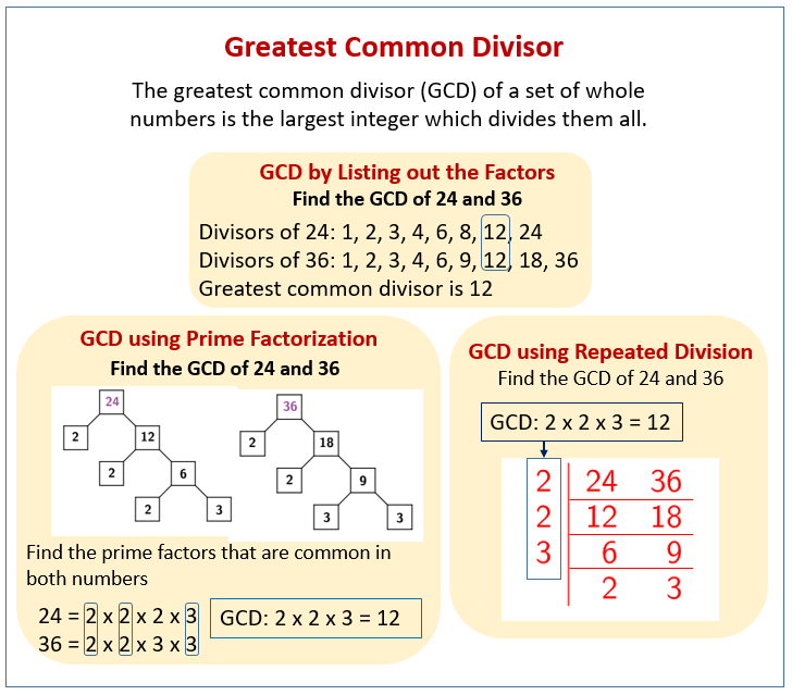
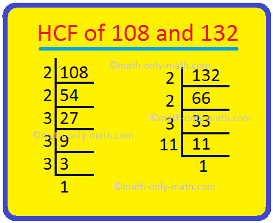
This method involves expressing numbers as products of prime numbers.

Example:

Find HCF of 36 and 48.

Prime factorization:

36 = 2 × 2 × 3 × 3
48 = 2 × 2 × 2 × 2 × 3

Common prime factors:

2 × 2 × 3

HCF = 12

Division Method

This method repeatedly divides numbers until a remainder appears.

Example:

Find HCF of 24 and 36.

36 ÷ 24 = 1 remainder 12

24 ÷ 12 = 2 remainder 0

HCF = 12

4. Understanding LCM (Least Common Multiple)

Definition

The Least Common Multiple (LCM) of two or more numbers is the smallest number that is a multiple of all the numbers.

Example:

Find LCM of 4 and 6.

Multiples of 4:

4, 8, 12, 16, 20…

Multiples of 6:

6, 12, 18, 24…

Common multiples:

12, 24…

Smallest common multiple:

LCM(4,6) = 12

5. Methods to Find LCM

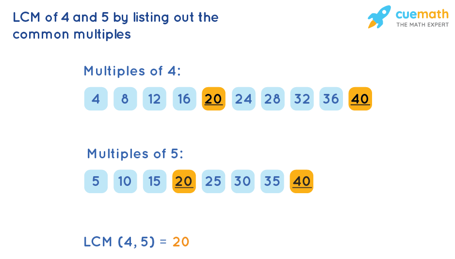
Listing Multiples Method

List multiples of each number and find the smallest common one.

Example:

LCM of 3 and 5

Multiples of 3:

3, 6, 9, 12, 15…

Multiples of 5:

5, 10, 15…

LCM = 15

Prime Factorization Method

Example:

Find LCM of 12 and 18.

Prime factorization:

12 = 2² × 3
18 = 2 × 3²

Take highest powers:

2² × 3²

LCM = 36

Division Method

Numbers are divided by prime numbers until all become 1.

Example:

Find LCM of 8 and 12.

8 = 2³
12 = 2² × 3

LCM = 2³ × 3

LCM = 24

6. Relationship Between LCM and HCF

There is an important relationship between LCM and HCF.

For two numbers:

LCM × HCF = Product of the numbers

Example:

Numbers = 12 and 18

HCF = 6
LCM = 36

Check:

36 × 6 = 216

12 × 18 = 216

Thus the relationship holds.

7. Prime Factorization and Number Theory

Prime factorization plays an important role in determining both LCM and HCF.

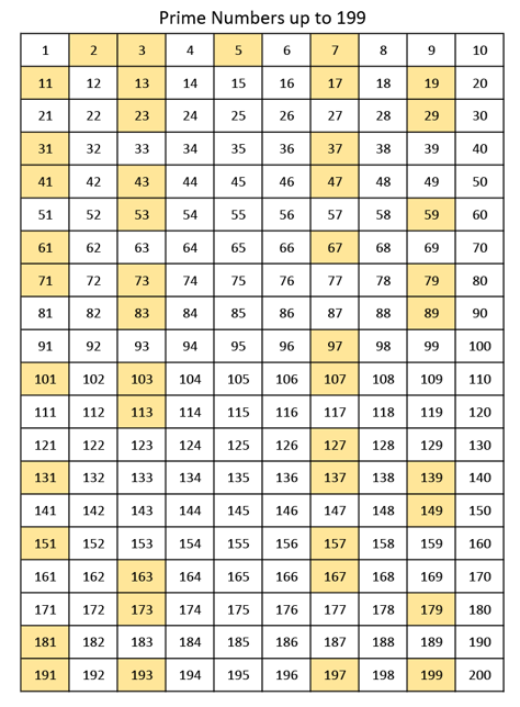
A prime number is a number that has only two factors:

1 and itself.

Examples:

2, 3, 5, 7, 11

Composite numbers can be expressed as products of primes.

Example:

60 = 2 × 2 × 3 × 5

This representation helps identify common factors and multiples easily.

8. Applications of HCF

HCF is useful in many mathematical and real-world situations.

Simplifying Fractions

Example:

12/18

HCF = 6

12 ÷ 6 = 2
18 ÷ 6 = 3

Simplified fraction:

2/3

Dividing Items Equally

Example:

24 apples and 36 oranges must be packed into equal baskets.

HCF = 12

Thus:

12 baskets can be formed.

Arranging Objects

HCF helps determine the largest group size when arranging objects evenly.

9. Applications of LCM

LCM is used when events repeat at regular intervals.

Scheduling Events

Example:

Two traffic lights change every 6 minutes and 8 minutes.

LCM of 6 and 8:

Both lights change together every 24 minutes.

Adding Fractions

LCM helps find common denominators.

Example:

1/4 + 1/6

LCM of 4 and 6 = 12

Convert:

3/12 + 2/12 = 5/12

Cyclic Events

LCM determines when repeating cycles align.

Example:

Two machines operate every 15 minutes and 20 minutes.

LCM = 60 minutes

10. LCM and HCF in Algebra

LCM and HCF are also applied to algebraic expressions.

Example:

Find LCM of:

x² and x³

LCM = x³

Example:

HCF of:

x²y and xy²

HCF = xy

These ideas are important when simplifying algebraic expressions.

11. Differences Between LCM and HCF

Feature	HCF	LCM
Meaning	Greatest common factor	Smallest common multiple
Focus	Factors	Multiples
Value	Smaller	Larger
Use	Simplification	Common denominators

12. Properties of HCF

Some important properties include:

HCF of two prime numbers is 1.

Example:

HCF(5,7) = 1

HCF of consecutive numbers is always 1.

Example:

HCF(8,9) = 1

HCF of identical numbers is the number itself.

Example:

HCF(12,12) = 12

13. Properties of LCM

Important properties include:

LCM of prime numbers is their product.

Example:

LCM(3,5) = 15

LCM of identical numbers is the number itself.

Example:

LCM(7,7) = 7

LCM of numbers always equals or exceeds the largest number.

14. Euclidean Algorithm

The Euclidean algorithm is an efficient method for finding HCF.

Procedure:

Divide the larger number by the smaller.
Replace the larger number with the smaller.
Replace the smaller number with the remainder.
Repeat until remainder becomes zero.

Example:

Find HCF of 48 and 18.

48 ÷ 18 = 2 remainder 12
18 ÷ 12 = 1 remainder 6
12 ÷ 6 = 2 remainder 0

HCF = 6

15. Importance of LCM and HCF

LCM and HCF are essential concepts in mathematics because they:

simplify calculations
help solve arithmetic problems
improve number understanding
support algebra and number theory

They also appear in computer science algorithms and engineering calculations.

16. Role in Computer Science

In computer science, LCM and HCF are used in:

cryptography
algorithm design
modular arithmetic
number theory algorithms

The Euclidean algorithm is one of the oldest and most efficient algorithms used in computing.

17. Role in Real-Life Problem Solving

These concepts help solve real-world problems involving:

time schedules
resource distribution
measurement conversions
engineering designs

Understanding LCM and HCF helps create efficient solutions.

18. Historical Development

The study of factors and multiples dates back to ancient mathematics.

Greek mathematicians studied divisibility and number relationships.

Euclid described methods for finding the greatest common divisor more than 2000 years ago.

These ideas remain fundamental in modern mathematics.

19. Advanced Topics Related to LCM and HCF

More advanced topics related to these concepts include:

number theory
modular arithmetic
Diophantine equations
cryptographic algorithms

These topics expand the study of factors and multiples in higher mathematics.

20. Summary

LCM and HCF are fundamental concepts in arithmetic and number theory. The Least Common Multiple helps identify the smallest common multiple of numbers, while the Highest Common Factor identifies the largest common divisor.

These concepts are essential for simplifying fractions, solving arithmetic problems, scheduling events, and analyzing numerical relationships.

Understanding LCM and HCF builds a strong foundation for more advanced topics in mathematics, including algebra, number theory, and computer science. Their applications extend beyond mathematics into everyday problem-solving and modern technology.

Percentages in Mathematics

Leave a reply

Tags:

Percentages in Mathematics

Percentages are one of the most widely used mathematical concepts in everyday life. The term percentage means “per hundred,” and it expresses a quantity as a fraction of 100. Percentages allow us to compare values, represent proportions, and interpret data in an easy and standardized form.

Percentages are used in various fields such as finance, economics, statistics, business, science, and education. From calculating discounts in stores to determining interest rates in banks, percentages play a critical role in real-world applications.

Understanding percentages also helps people interpret statistical information, analyze changes in quantities, and make informed decisions based on numerical data.

In mathematics, percentages are closely related to fractions and decimals, and they can easily be converted between these different numerical forms.

1. Definition of Percentage

A percentage is a number expressed as a fraction of 100.

The word percentage comes from the Latin phrase “per centum,” which means “out of one hundred.”

The symbol used for percentage is:

For example:

25% means 25 out of 100.

Mathematically:

25% = 25/100

This can also be written as:

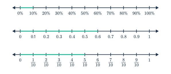
0.25

Thus, percentages can be represented in three forms:

fraction
decimal
percent

2. Understanding Percentages

Percentages represent parts of a whole where the whole equals 100.

Example:

If 60 out of 100 students passed an exam, the percentage of students who passed is:

60%

This means 60 parts out of 100.

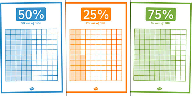
Visual Interpretation

Percentages are often illustrated using diagrams such as:

pie charts
bar charts
grids with 100 squares

For example:

50% of a pie chart represents half of the circle.

75% represents three quarters of the circle.

These visual models help people easily understand proportions.

3. Converting Between Fractions, Decimals, and Percentages

Percentages can easily be converted into fractions and decimals.

Percentage to Fraction

To convert a percentage to a fraction:

Write the percentage over 100 and simplify.

Example:

40%

40/100

Simplified:

2/5

Percentage to Decimal

To convert a percentage to a decimal:

Divide by 100.

Example:

75%

75 ÷ 100 = 0.75

Fraction to Percentage

Multiply the fraction by 100.

Example:

1/4

1/4 × 100 = 25%

Decimal to Percentage

Multiply the decimal by 100.

Example:

0.6

0.6 × 100 = 60%

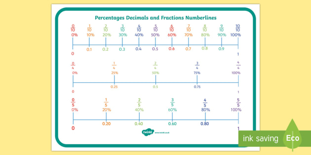
4. Common Percentage Values

Some percentages are commonly used and easily recognized.

Percentage	Fraction	Decimal
50%	1/2	0.5
25%	1/4	0.25
75%	3/4	0.75
10%	1/10	0.1
20%	1/5	0.2

These values frequently appear in everyday calculations.

5. Calculating Percentages

The basic formula for calculating a percentage is:

Percentage = (Part / Whole) × 100

Example

Suppose a class has 40 students, and 30 passed the exam.

Part = 30
Whole = 40

Percentage = (30/40) × 100

Percentage = 75%

Thus, 75% of students passed the exam.

6. Finding a Percentage of a Number

To find a percentage of a number:

Convert the percentage to decimal and multiply.

Example:

Find 20% of 150.

Step 1:

20% = 0.20

Step 2:

0.20 × 150 = 30

Answer:

Example:

Find 15% of 200.

15% = 0.15

0.15 × 200 = 30

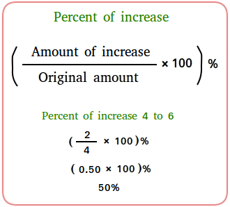
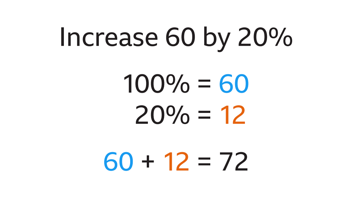
7. Percentage Increase

Percentage increase measures how much a quantity grows compared to its original value.

Formula:

Percentage Increase = (Increase / Original Value) × 100

Example

Original price = $50
New price = $65

Increase:

65 − 50 = 15

Percentage increase:

(15/50) × 100 = 30%

Thus, the price increased by 30%.

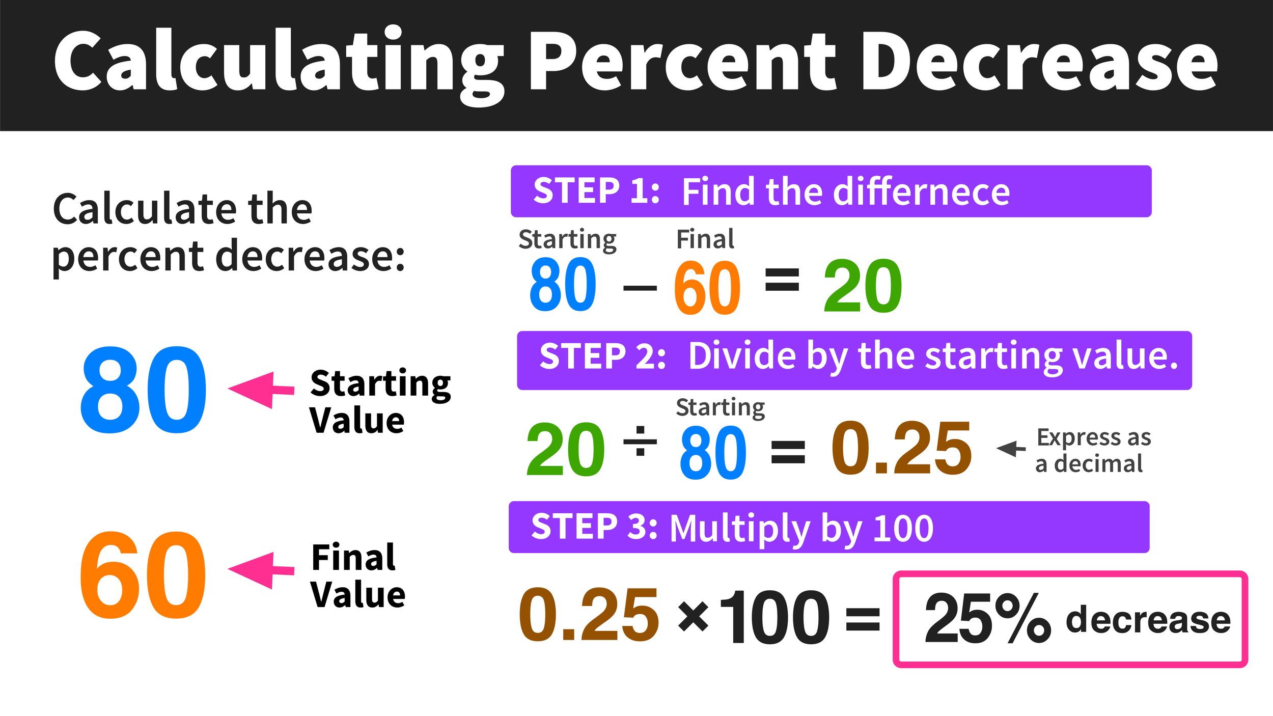
8. Percentage Decrease

Percentage decrease measures how much a quantity decreases relative to the original value.

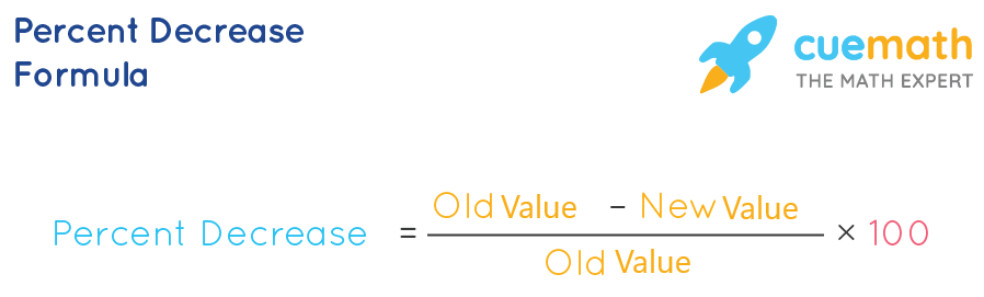
Formula:

Percentage Decrease = (Decrease / Original Value) × 100

Example

Original value = 80
New value = 60

Decrease:

80 − 60 = 20

Percentage decrease:

(20/80) × 100 = 25%

Thus, the value decreased by 25%.

9. Percentage Change

Percentage change describes the overall change between two values.

Formula:

Percentage Change = (New Value − Original Value / Original Value) × 100

This value may be positive (increase) or negative (decrease).

10. Applications of Percentages

Percentages are widely used in real-world situations.

Discounts in Shopping

Stores often offer discounts using percentages.

Example:

20% discount on a $100 item.

Discount amount:

20% of 100 = 20

New price:

100 − 20 = 80

Banking and Interest

Banks use percentages to calculate interest rates.

Example:

5% annual interest on savings.

Taxes

Governments use percentage rates to calculate taxes.

Example:

10% sales tax.

Statistics

Percentages help interpret data.

Example:

Population growth rates.

Education

Grades are often expressed as percentages.

Example:

85% score on an exam.

11. Percentage in Data Representation

Percentages are commonly used in data visualization.

Common charts include:

pie charts
bar graphs
percentage grids

Example:

If 40% of people prefer tea and 60% prefer coffee, a pie chart clearly shows the difference.

These visualizations help communicate information effectively.

12. Percentages in Business

Businesses rely heavily on percentage calculations.

Examples include:

profit percentage
loss percentage
growth rate
market share

Profit Percentage

Profit percentage formula:

Profit % = (Profit / Cost Price) × 100

Loss Percentage

Loss % = (Loss / Cost Price) × 100

13. Percentages in Science

In science, percentages are used to express concentrations.

Examples:

chemical solutions
humidity
probability

Example:

A solution may contain 10% salt.

14. Percentages in Probability

Probability is often expressed as a percentage.

Example:

If the probability of rain is 0.3:

0.3 × 100 = 30%

Thus, there is a 30% chance of rain.

15. Percentages in Economics

Economists use percentages to analyze financial trends.

Examples include:

inflation rates
unemployment rates
economic growth rates

These percentages help governments make economic decisions.

16. Importance of Percentages in Mathematics

Percentages are important because they:

simplify comparisons
express proportions clearly
help analyze data
support decision making

They also form the basis for advanced topics such as statistics and finance.

17. Historical Background of Percentages

The concept of percentages developed through trade and commerce.

Merchants needed a standardized way to express:

profit margins
interest rates
tax calculations

Over time, percentages became a universal mathematical tool used worldwide.

18. Relationship with Ratios and Proportions

Percentages are closely related to ratios and proportions.

Example:

25%

This represents the ratio:

25 : 100

Which simplifies to:

1 : 4

Thus, percentages can be viewed as ratios with denominator 100.

19. Percentage Errors

Percentage error measures how close a measured value is to the true value.

Formula:

Percentage Error = (|Measured − True| / True) × 100

Example:

True value = 100
Measured value = 95

Error:

Percentage error:

This concept is widely used in scientific experiments.

20. Summary

Percentages are a fundamental mathematical concept used to represent proportions out of one hundred. They provide a convenient and universal way to compare quantities, analyze data, and express numerical relationships.

Percentages can easily be converted into fractions and decimals, making them flexible tools in mathematics. They are used extensively in everyday activities such as shopping, banking, education, and statistics.

In mathematics and science, percentages help interpret information, measure changes, and communicate data clearly. Their widespread applications make them one of the most practical and essential concepts in both academic study and real-world problem solving.

Ratios and Proportions in Mathematics

Leave a reply

Tags:

Ratios and Proportions in Mathematics

Ratios and proportions are fundamental mathematical concepts used to compare quantities and describe relationships between numbers. These concepts are widely used in everyday life, science, engineering, economics, and many other fields.

A ratio expresses the relationship between two quantities, indicating how many times one value contains or is contained within another. A proportion, on the other hand, states that two ratios are equal.

Ratios and proportions are essential tools for solving problems involving scaling, mixing, measurements, rates, and comparisons. They also form the foundation for advanced topics such as algebra, trigonometry, statistics, and calculus.

Understanding ratios and proportions helps people interpret real-world data, perform calculations, and make logical comparisons between quantities.

1. Understanding Ratios

Definition of a Ratio

A ratio is a mathematical expression used to compare two quantities.

A ratio shows how many times one value is contained in another.

For example, if there are:

4 apples
2 oranges

The ratio of apples to oranges is:

4 : 2

This means there are 4 apples for every 2 oranges.

Ways to Write Ratios

Ratios can be written in three common forms:

Using a colon
3 : 5
Using the word “to”
3 to 5
As a fraction
3/5

All three forms represent the same ratio.

Terms in a Ratio

In a ratio a : b:

a is called the antecedent
b is called the consequent

Example:

In the ratio 4 : 7

4 is the antecedent
7 is the consequent

2. Simplifying Ratios

Ratios can often be simplified in the same way as fractions.

Example:

6 : 8

Divide both numbers by their greatest common divisor.

GCD of 6 and 8 = 2

6 ÷ 2 = 3
8 ÷ 2 = 4

Simplified ratio:

3 : 4

Simplifying ratios makes comparisons easier to understand.

3. Types of Ratios

Ratios can appear in different forms depending on what is being compared.

Part-to-Part Ratio

A part-to-part ratio compares two different parts of a group.

Example:

In a class:

10 boys
15 girls

Ratio of boys to girls:

10 : 15

Simplified:

2 : 3

Part-to-Whole Ratio

A part-to-whole ratio compares one part to the total.

Example:

Total students = 25

Boys = 10

Ratio of boys to total students:

10 : 25

Simplified:

2 : 5

4. Equivalent Ratios

Equivalent ratios represent the same relationship between numbers.

Example:

2 : 3

Equivalent ratios include:

4 : 6
6 : 9
8 : 12

These ratios are obtained by multiplying both terms by the same number.

Example:

2 × 2 = 4
3 × 2 = 6

Equivalent ratios are important when solving proportion problems.

5. Understanding Proportions

Definition of Proportion

A proportion is an equation stating that two ratios are equal.

Example:

2/3 = 4/6

This shows that the two ratios represent the same relationship.

Proportions are used to solve problems involving unknown quantities.

Structure of a Proportion

A proportion has four numbers.

Example:

a/b = c/d

Here:

a and d are called extremes
b and c are called means

Cross Multiplication

Cross multiplication is used to solve proportions.

Example:

3/4 = x/8

Cross multiply:

3 × 8 = 4 × x

24 = 4x

x = 6

6. Direct Proportion

Two quantities are in direct proportion when one increases or decreases in the same ratio as the other.

Mathematically:

y = kx

Where k is the constant of proportionality.

Example of Direct Proportion

If one notebook costs $2:

1 notebook = $2
2 notebooks = $4
3 notebooks = $6

Cost is directly proportional to the number of notebooks.

Graph of Direct Proportion

The graph of a direct proportion is a straight line passing through the origin.

7. Inverse Proportion

Two quantities are in inverse proportion when one increases while the other decreases.

Mathematical relationship:

xy = k

Where k is a constant.

Example of Inverse Proportion

If 4 workers complete a job in 6 hours:

More workers reduce time.

Example:

4 workers → 6 hours
6 workers → 4 hours

Workers and time are inversely proportional.

8. Continued Proportion

When three numbers are in proportion such that:

a : b = b : c

They form a continued proportion.

Example:

2 : 4 = 4 : 8

Here:

4 is the mean proportional.

9. Compound Ratio

A compound ratio is obtained by multiplying two or more ratios.

Example:

2 : 3 and 4 : 5

Compound ratio:

(2×4) : (3×5)

8 : 15

Compound ratios are used in complex comparisons.

10. Applications of Ratios

Ratios appear in many real-life situations.

Cooking

Recipes often use ratios.

Example:

2 cups flour : 1 cup sugar

This ratio maintains flavor balance.

Maps and Scale

Maps use ratios to represent distances.

Example:

1 cm : 10 km

This means 1 cm on the map equals 10 km in reality.

Mixing Solutions

Chemistry uses ratios when mixing substances.

Example:

Water to chemical ratio.

Finance

Ratios are used to compare financial quantities.

Examples include:

profit ratios
interest rates
investment comparisons

Sports Statistics

Ratios are used to evaluate performance.

Example:

Goals per game.

11. Applications of Proportions

Proportions help solve many practical problems.

Speed and Distance

Example:

If a car travels 60 km in 1 hour:

Distance is proportional to time.

Currency Conversion

Exchange rates use proportions.

Example:

1 USD = 80 INR

Construction

Architects use proportional scaling when designing buildings.

Photography

Aspect ratios determine image dimensions.

Example:

16 : 9

12. Ratio Tables

A ratio table lists pairs of values that maintain a constant ratio.

Example:

Apples	Oranges
2	3
4	6
6	9

Each pair represents the same ratio.

Ratio tables help visualize proportional relationships.

13. Unit Rate

A unit rate expresses a ratio with denominator 1.

Example:

60 km in 2 hours

Unit rate:

30 km per hour

Unit rates simplify comparisons.

14. Ratios and Fractions

Ratios are closely related to fractions.

Example:

2 : 5 = 2/5

Fractions express part-to-whole relationships, while ratios compare quantities.

15. Ratios and Percentages

Percentages are ratios with denominator 100.

Example:

25%

25/100

1/4

Percentages allow easy comparison of proportions.

16. Importance in Mathematics

Ratios and proportions are fundamental in mathematics because they describe relationships between numbers.

They are used in:

algebra
geometry
trigonometry
statistics

Many mathematical formulas rely on proportional relationships.

17. Role in Science and Engineering

In science and engineering, ratios and proportions help describe relationships between variables.

Examples include:

density
speed
concentration
electrical resistance

These relationships allow scientists and engineers to model real-world systems.

18. Ratio and Proportion in Data Analysis

In statistics, ratios help interpret data.

Examples:

population ratios
probability ratios
risk ratios

These measurements help analyze trends and relationships.

19. Historical Development

The study of ratios and proportions dates back to ancient civilizations.

Greek mathematicians studied proportional relationships in geometry.

These ideas were later developed into formal mathematical theories used in modern mathematics.

20. Summary

Ratios and proportions are essential mathematical tools used to compare quantities and describe relationships between numbers.

A ratio compares two quantities, while a proportion states that two ratios are equal.

These concepts appear in many real-world applications, including cooking, construction, finance, science, and engineering.

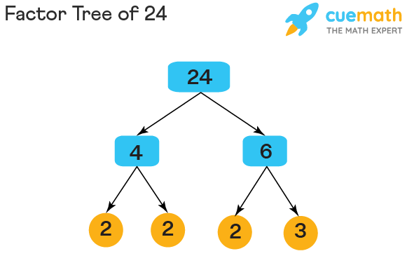
Understanding ratios and proportions helps build strong mathematical reasoning and prepares students for advanced topics in mathematics and science.

They remain fundamental tools for analyzing relationships, solving problems, and interpreting numerical information.

Fractions and Decimals in Mathematics

Leave a reply

Tags:

Fractions and Decimals in Mathematics

Fractions and decimals are essential concepts in mathematics that represent numbers that are not whole numbers. They are used to express parts of a whole, ratios, proportions, and precise measurements. These forms of numbers belong to a broader class called rational numbers, which can be expressed as the ratio of two integers.

Fractions and decimals are widely used in everyday life, including in finance, measurements, engineering, science, and computer calculations. Understanding how fractions and decimals work allows us to perform precise calculations and interpret numerical data more effectively.

In mathematics, fractions represent numbers in the form of a ratio of two integers, while decimals represent numbers using the base-10 positional number system. Both representations can often express the same value, and there are methods to convert between them.

Fractions and decimals are taught early in mathematics education because they form the foundation for algebra, statistics, calculus, and other advanced mathematical topics.

1. Understanding Fractions

Definition of a Fraction

A fraction represents a part of a whole or a ratio between two quantities.

A fraction is written in the form:

a/b

Where:

a is called the numerator
b is called the denominator

Example:

3/4

This means 3 parts out of 4 equal parts.

Example interpretation:

If a pizza is divided into 4 equal slices and you eat 3 slices, you have eaten 3/4 of the pizza.

Parts of a Fraction

Every fraction has two main components:

Numerator

The number on the top.

It represents how many parts are being considered.

Example:

In 5/8, the numerator is 5.

Denominator

The number on the bottom.

It represents the total number of equal parts.

Example:

In 5/8, the denominator is 8.

2. Types of Fractions

Fractions can be categorized into several types depending on their structure.

Proper Fractions

A proper fraction has a numerator smaller than the denominator.

Example:

1/2
3/5
7/8

In these fractions, the value is always less than 1.

Improper Fractions

An improper fraction has a numerator greater than or equal to the denominator.

Example:

5/3
9/4
7/7

Improper fractions represent values greater than or equal to 1.

Mixed Fractions

A mixed fraction combines a whole number and a proper fraction.

Example:

2 1/3

This means:

2 + 1/3

Mixed numbers are often used in everyday measurements.

Example:

2 1/2 meters

Equivalent Fractions

Equivalent fractions represent the same value even though their numerators and denominators differ.

Example:

1/2 = 2/4 = 4/8

These fractions represent the same portion of a whole.

Equivalent fractions are obtained by multiplying or dividing both numerator and denominator by the same number.

Example:

1/2 × 2/2 = 2/4

3. Simplifying Fractions

Simplifying (or reducing) a fraction means expressing it in its lowest terms.

Example:

6/8

Both numbers can be divided by 2:

6 ÷ 2 = 3
8 ÷ 2 = 4

Simplified fraction:

3/4

To simplify fractions, we divide numerator and denominator by their greatest common divisor (GCD).

Example:

15/25

GCD of 15 and 25 = 5

15 ÷ 5 = 3
25 ÷ 5 = 5

Simplified form:

3/5

4. Comparing Fractions

Fractions can be compared to determine which is larger or smaller.

Example:

3/4 and 2/3

Convert them to a common denominator.

Common denominator = 12

3/4 = 9/12
2/3 = 8/12

Therefore:

3/4 > 2/3

Fractions can also be compared using decimal conversions.

5. Operations on Fractions

Fractions support four basic arithmetic operations.

Addition of Fractions

To add fractions with the same denominator:

Add numerators and keep denominator.

Example:

2/7 + 3/7 = 5/7

For different denominators, find a common denominator.

Example:

1/3 + 1/4

Common denominator = 12

1/3 = 4/12
1/4 = 3/12

Sum:

7/12

Subtraction of Fractions

Similar to addition.

Example:

5/6 − 1/3

Convert:

1/3 = 2/6

Result:

3/6 = 1/2

Multiplication of Fractions

Multiply numerators and denominators.

Example:

2/3 × 4/5

Result:

8/15

Division of Fractions

Division involves multiplying by the reciprocal.

Example:

3/4 ÷ 2/5

Convert:

3/4 × 5/2

Result:

15/8

6. Understanding Decimals

Definition of Decimals

A decimal is a number expressed in the base-10 system using a decimal point.

Example:

0.5
1.25
3.75

Decimals represent fractional values using place value.

Decimal Place Value

Decimal numbers extend the place value system to the right of the decimal point.

Example:

4.375

Place values:

4 → ones
3 → tenths
7 → hundredths
5 → thousandths

Decimal Place Value Table

Place	Value
Ones	1
Tenths	0.1
Hundredths	0.01
Thousandths	0.001

7. Types of Decimals

Decimals can be categorized into different types.

Terminating Decimals

Decimals that end after a finite number of digits.

Example:

0.5
0.25
0.125

These correspond to fractions with denominators that are powers of 2 or 5.

Example:

1/2 = 0.5

Non-Terminating Decimals

Decimals that continue indefinitely.

Example:

1/3 = 0.333…

Repeating Decimals

Decimals with repeating patterns.

Example:

0.666…

This is written as:

0.6̅

8. Converting Fractions to Decimals

Fractions can be converted into decimals by dividing numerator by denominator.

Example:

1/4

1 ÷ 4 = 0.25

Another example:

3/8

3 ÷ 8 = 0.375

Some fractions produce repeating decimals.

Example:

1/3

0.333…

9. Converting Decimals to Fractions

Decimals can also be converted to fractions.

Example:

0.75

Step 1:

Write as fraction:

75/100

Step 2:

Simplify:

3/4

Example:

0.2

2/10 = 1/5

10. Operations with Decimals

Decimals support the same arithmetic operations as whole numbers.

Addition

Example:

2.35 + 1.40

Align decimal points:

3.75

Subtraction

Example:

5.6 − 2.3

Result:

3.3

Multiplication

Example:

2.5 × 1.2

25 × 12 = 300

Decimal places = 2

Result:

3.00

Division

Example:

4.8 ÷ 2

Result:

2.4

11. Relationship Between Fractions and Decimals

Fractions and decimals represent the same numbers in different formats.

Examples:

1/2 = 0.5
1/4 = 0.25
3/5 = 0.6

Fractions emphasize ratio, while decimals emphasize place value.

12. Fractions and Decimals on a Number Line

Fractions and decimals can be represented visually on a number line.

Example:

0 — 1

Halfway point:

1/2 or 0.5

Other examples:

1/4 = 0.25
3/4 = 0.75

The number line helps visualize magnitude and relationships between numbers.

13. Applications of Fractions and Decimals

Fractions and decimals are used in many real-life contexts.

Measurements

Fractions and decimals represent measurements.

Example:

1/2 meter
0.75 kilogram

Finance

Decimals are widely used in money.

Example:

$5.75

Cooking

Recipes use fractions.

Example:

1/2 cup
3/4 teaspoon

Engineering

Precise measurements use decimals.

Example:

2.35 millimeters

Science

Scientific calculations often use decimal numbers.

Example:

9.81 m/s²

14. Importance in Mathematics

Fractions and decimals are essential for many mathematical topics.

They form the foundation for:

ratios and proportions
percentages
algebra
statistics
calculus

Without fractions and decimals, it would be difficult to express precise values.

15. Summary

Fractions and decimals are important numerical representations used to express values between whole numbers.

Fractions represent numbers as ratios of integers, while decimals represent numbers using the base-10 positional system.

Understanding fractions and decimals involves learning their types, conversions, arithmetic operations, and practical applications.

These concepts are fundamental to mathematics, science, engineering, finance, and everyday life.

Mastery of fractions and decimals allows for accurate calculations, better numerical understanding, and deeper insight into more advanced mathematical ideas.