Category Archives: Mathematics

Transformations in Geometry (Reflection, Rotation, Translation)

Image
Image
Image
Image

Introduction to Geometric Transformations

In mathematics, transformations describe how a geometric figure changes its position, orientation, or size in a plane. Transformations are fundamental concepts in geometry because they help us understand how shapes move and how they relate to each other.

A transformation maps every point of a figure to a new position according to a specific rule. When a transformation occurs, the original figure is called the pre-image, and the resulting figure after transformation is called the image.

Transformations play an important role in many mathematical topics such as coordinate geometry, symmetry, congruence, and similarity. They are also widely used in fields like computer graphics, engineering design, robotics, physics, architecture, and animation.

The most common types of geometric transformations are:

  • Translation
  • Reflection
  • Rotation
  • Dilation

However, the three most basic transformations studied in geometry are translation, reflection, and rotation. These transformations preserve the size and shape of figures and are therefore called rigid transformations or isometries.


Definition of Transformation

A transformation is a mathematical operation that moves or changes a geometric figure in a plane according to certain rules.

The transformation assigns each point ((x,y)) of the original figure to a new point ((x’,y’)).

The transformation can change:

  • the position of a shape
  • the orientation of a shape
  • the direction of a shape

But rigid transformations do not change the size or shape of the figure.


Types of Transformations

The three main types of transformations studied in geometry are:

  1. Translation
  2. Reflection
  3. Rotation

Each transformation moves the figure in a different way.


Translation

Definition of Translation

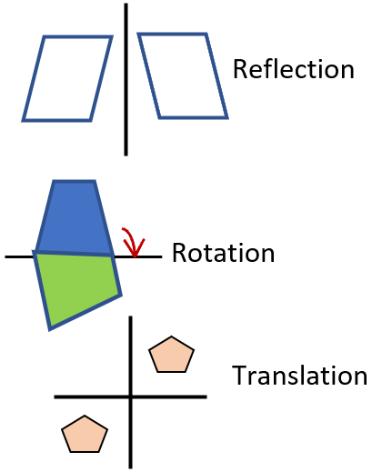
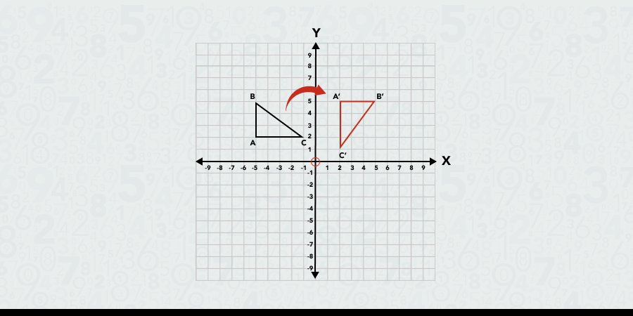
A translation is a transformation that moves every point of a figure the same distance in the same direction.

In translation:

  • The shape does not rotate.
  • The shape does not change size.
  • The orientation remains the same.

Translation is often described as a slide.


Example of Translation

Consider a point:

[
(2,3)
]

If we translate the point 4 units right and 2 units up:

[
(2+4, 3+2)
]

[
(6,5)
]

The new point becomes (6,5).


Translation Rule

Translation can be expressed using coordinate rules.

General rule:

[
(x,y) \rightarrow (x+a, y+b)
]

Where:

  • (a) = horizontal movement
  • (b) = vertical movement

Example:

[
(x,y) \rightarrow (x+3,y-2)
]

Means move:

  • 3 units right
  • 2 units down

Properties of Translation

Important properties include:

  • Distance between points remains the same
  • Angles remain unchanged
  • Shape and size remain unchanged
  • Orientation stays the same

Translation preserves congruence.


Reflection

Definition of Reflection

A reflection is a transformation that flips a figure over a line called the line of reflection.

Reflection produces a mirror image of the original figure.

The line of reflection acts like a mirror.


Example of Reflection

If a point lies on one side of the mirror line, the reflected point appears the same distance on the opposite side.

Example:

Point:

[
(3,4)
]

Reflection across the y-axis:

[
(-3,4)
]


Reflection Rules

Reflection Across X-axis

Rule:

[
(x,y) \rightarrow (x,-y)
]

Example:

[
(2,5) \rightarrow (2,-5)
]


Reflection Across Y-axis

Rule:

[
(x,y) \rightarrow (-x,y)
]

Example:

[
(3,4) \rightarrow (-3,4)
]


Reflection Across Origin

Rule:

[
(x,y) \rightarrow (-x,-y)
]


Reflection Across Line (y=x)

Rule:

[
(x,y) \rightarrow (y,x)
]


Properties of Reflection

Reflection preserves:

  • shape
  • size
  • distance

However, orientation is reversed.

For example, clockwise order becomes counterclockwise.


Rotation

Definition of Rotation

A rotation is a transformation that turns a figure around a fixed point called the center of rotation.

The rotation occurs through a certain angle and in a certain direction.

Rotations can be:

  • clockwise
  • counterclockwise

Center of Rotation

The center of rotation is the fixed point around which the figure rotates.

Often, rotations occur around the origin (0,0).


Common Rotation Angles

Common rotation angles include:

  • 90°
  • 180°
  • 270°

Rotation Rules

90° Counterclockwise Rotation

Rule:

[
(x,y) \rightarrow (-y,x)
]

Example:

[
(3,2) \rightarrow (-2,3)
]


180° Rotation

Rule:

[
(x,y) \rightarrow (-x,-y)
]

Example:

[
(4,5) \rightarrow (-4,-5)
]


270° Counterclockwise Rotation

Rule:

[
(x,y) \rightarrow (y,-x)
]

Example:

[
(2,3) \rightarrow (3,-2)
]


Properties of Rotation

Rotation preserves:

  • shape
  • size
  • distance
  • angle measures

However, the orientation of the figure may change depending on the rotation.


Rigid Transformations

Translation, reflection, and rotation are called rigid transformations.

They preserve:

  • length
  • angle
  • area
  • shape

Because of this property, the original and transformed figures are congruent.


Composition of Transformations

Sometimes multiple transformations are applied in sequence.

This is called a composition of transformations.

Example:

  1. Translate a triangle.
  2. Rotate it 90°.
  3. Reflect it across the y-axis.

The final position depends on the order of transformations.


Transformations in Coordinate Geometry

Transformations are often studied using coordinate geometry.

Each transformation can be described using coordinate rules.

Example:

Triangle with vertices:

[
A(1,2), B(3,2), C(2,4)
]

After translation by (2,1):

[
A'(3,3), B'(5,3), C'(4,5)
]


Symmetry and Transformations

Transformations are closely related to symmetry.

Example:

Reflection symmetry occurs when a shape is mirrored.

Rotation symmetry occurs when a shape looks the same after rotation.

Example shapes with symmetry:

  • square
  • equilateral triangle
  • circle

Transformations in Real Life

Transformations appear in many real-world applications.


Computer Graphics

Computer graphics use transformations to move objects on the screen.

Example:

Video game characters are translated, rotated, and reflected.


Robotics

Robots use transformations to calculate movement paths.


Architecture

Architectural designs often involve symmetrical reflections and rotations.


Physics

Physics uses transformations to describe motion and coordinate systems.


Animation

Animation relies heavily on transformations to move objects smoothly.


Transformations in Art and Design

Artists and designers use geometric transformations to create patterns.

Examples include:

  • tessellations
  • tiling designs
  • decorative patterns

Mathematical Representation of Transformations

Transformations can also be represented using matrices.

Matrix transformations are used in:

  • computer graphics
  • physics simulations
  • 3D modeling

Example:

Rotation matrices represent rotations in coordinate space.


Transformations in Higher Dimensions

Transformations are not limited to two dimensions.

In 3D space, transformations include:

  • rotations around axes
  • reflections across planes
  • translations in space

These transformations are used in:

  • virtual reality
  • robotics
  • mechanical simulations

Importance of Transformations

Transformations are important because they:

  • help analyze geometric relationships
  • explain symmetry
  • support coordinate geometry
  • model motion and movement

They also connect geometry with algebra and linear algebra.


Historical Development

The study of transformations developed alongside geometry.

Ancient mathematicians studied symmetry and reflections.

In modern mathematics, transformation geometry became an important field that focuses on geometric transformations and their properties.


Conclusion

Transformations in geometry describe how shapes move or change position within a coordinate plane. The three primary transformations—translation, reflection, and rotation—are fundamental tools for understanding geometric relationships and symmetry.

Translation slides a figure from one location to another without changing its orientation. Reflection flips a figure across a line, creating a mirror image. Rotation turns a figure around a fixed point by a specified angle.

These transformations preserve the size and shape of figures, making them rigid transformations. They play a crucial role in mathematics and have applications in many fields such as computer graphics, engineering, physics, architecture, and animation.

By studying transformations, mathematicians gain deeper insights into geometric structures and spatial relationships, making transformation geometry an essential part of mathematical education and modern scientific applications.


Tags

Coordinate Geometry

Image
Image
Image
Image

Introduction to Coordinate Geometry

Coordinate geometry, also known as analytic geometry, is a branch of mathematics that combines algebra and geometry to study geometric figures using a coordinate system. In this system, points are represented by numerical coordinates that describe their position in a plane.

The development of coordinate geometry revolutionized mathematics by allowing geometric problems to be solved using algebraic equations. This approach makes it easier to analyze shapes, calculate distances, determine slopes, and represent curves.

Coordinate geometry is widely used in mathematics, physics, engineering, computer science, navigation, and many other scientific fields. It provides a powerful framework for understanding spatial relationships and solving problems involving geometric figures.

The most common coordinate system used in coordinate geometry is the Cartesian coordinate system, which uses two perpendicular axes to locate points in a plane.


Historical Background

Coordinate geometry was developed in the 17th century by the French mathematician René Descartes. His work established a method of representing geometric shapes using algebraic equations.

Before Descartes introduced this concept, geometry and algebra were treated as separate branches of mathematics. By combining them, Descartes created a powerful mathematical tool that allowed curves and shapes to be analyzed using equations.

The Cartesian coordinate system was named after Descartes in recognition of his contribution to mathematics.


Cartesian Coordinate System

The Cartesian coordinate system consists of two perpendicular number lines called axes.

These axes intersect at a point called the origin.

The horizontal axis is called the x-axis.

The vertical axis is called the y-axis.

The point where the axes intersect is represented as:

[
(0,0)
]

This point is called the origin.


Axes of the Coordinate Plane

The coordinate plane consists of two axes.

X-axis

The x-axis is the horizontal axis.

It represents horizontal movement across the plane.


Y-axis

The y-axis is the vertical axis.

It represents vertical movement.


Coordinates of a Point

Every point in the coordinate plane is represented by an ordered pair.

The ordered pair is written as:

[
(x,y)
]

Where:

  • (x) is the horizontal coordinate
  • (y) is the vertical coordinate

Example:

[
(3,4)
]

This means the point lies:

  • 3 units along the x-axis
  • 4 units along the y-axis

Quadrants of the Coordinate Plane

The coordinate plane is divided into four regions called quadrants.


First Quadrant

Both coordinates are positive.

[
(+,+)
]

Example:

(4,5)


Second Quadrant

x is negative, y is positive.

[
(-,+)
]

Example:

(-3,4)


Third Quadrant

Both coordinates are negative.

[
(-,-)
]

Example:

(-5,-2)


Fourth Quadrant

x is positive, y is negative.

[
(+,-)
]

Example:

(4,-3)


Plotting Points

Plotting points involves locating coordinates on the plane.

Steps:

  1. Start at the origin.
  2. Move along the x-axis according to the x-value.
  3. Move vertically according to the y-value.
  4. Mark the point.

Example:

Point (2,3)

Move 2 units right, then 3 units up.


Distance Between Two Points

One of the most important formulas in coordinate geometry is the distance formula.

For two points:

[
(x_1,y_1) \quad and \quad (x_2,y_2)
]

Distance:

[
d = \sqrt{(x_2-x_1)^2 + (y_2-y_1)^2}
]

This formula is derived from the Pythagorean theorem.


Example of Distance Formula

Points:

[
(1,2) \quad and \quad (4,6)
]

Distance:

[
d = \sqrt{(4-1)^2 + (6-2)^2}
]

[
d = \sqrt{9 + 16}
]

[
d = \sqrt{25}
]

[
d = 5
]


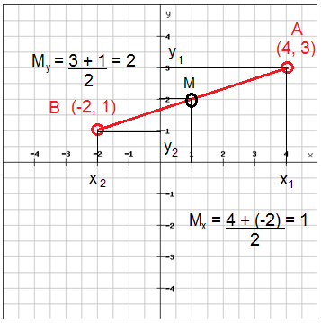
Midpoint Formula

The midpoint of a line segment is the point that divides the segment into two equal parts.

Formula:

[
M = \left(\frac{x_1+x_2}{2}, \frac{y_1+y_2}{2}\right)
]


Example of Midpoint

Points:

[
(2,4) \quad and \quad (6,8)
]

Midpoint:

[
M = (4,6)
]


Slope of a Line

The slope measures how steep a line is.

Formula:

[
m = \frac{y_2 – y_1}{x_2 – x_1}
]

Slope represents the rate of change between two points.


Types of Slopes

Lines can have different types of slopes.


Positive Slope

Line rises from left to right.

Example:

(m > 0)


Negative Slope

Line falls from left to right.

Example:

(m < 0)


Zero Slope

Horizontal line.

Example:

(m = 0)


Undefined Slope

Vertical line.

Division by zero occurs.


Equation of a Line

Lines in coordinate geometry are represented by equations.


Slope-Intercept Form

[
y = mx + c
]

Where:

  • (m) = slope
  • (c) = y-intercept

Example

[
y = 2x + 3
]

Slope = 2
Y-intercept = 3


Point-Slope Form

[
y – y_1 = m(x – x_1)
]

Used when slope and one point are known.


Two-Point Form

Used when two points are known.

[
y-y_1 = \frac{y_2-y_1}{x_2-x_1}(x-x_1)
]


Intercept Form

[
\frac{x}{a} + \frac{y}{b} = 1
]

Where:

  • (a) = x-intercept
  • (b) = y-intercept

Parallel Lines

Two lines are parallel if they have the same slope.

Example:

[
y = 3x + 1
]

[
y = 3x – 4
]

Both have slope 3.


Perpendicular Lines

Two lines are perpendicular if the product of their slopes equals -1.

Example:

If:

[
m_1 = 2
]

Then:

[
m_2 = -\frac{1}{2}
]


Area of Triangle in Coordinate Geometry

Area formula using coordinates:

[
A = \frac{1}{2} |x_1(y_2-y_3)+x_2(y_3-y_1)+x_3(y_1-y_2)|
]


Equation of a Circle

Circle equation in coordinate geometry:

[
(x-h)^2 + (y-k)^2 = r^2
]

Where:

  • (h,k) = center
  • r = radius

Graphs of Functions

Coordinate geometry allows functions to be represented graphically.

Example:

[
y = x^2
]

This produces a parabola.


Transformations in Coordinate Geometry

Graphs can be transformed by shifting, stretching, or reflecting.

Example:

[
y = (x-2)^2
]

Shifted right by 2 units.


Applications of Coordinate Geometry

Coordinate geometry has many practical applications.


Engineering

Used in structural design and mechanical systems.


Physics

Used to analyze motion and forces.


Computer Graphics

Digital images and animations rely heavily on coordinate geometry.


Navigation

GPS systems use coordinates to determine location.


Robotics

Robot movements are calculated using coordinate systems.


Architecture

Building layouts are designed using coordinate-based plans.


Coordinate Geometry in Calculus

In calculus, coordinate geometry helps analyze curves.

Concepts include:

  • derivatives
  • integrals
  • limits

Curves are described using equations in the coordinate plane.


Three-Dimensional Coordinate Geometry

Beyond two dimensions, coordinate systems extend into 3D space.

Coordinates are written as:

[
(x,y,z)
]

Axes include:

  • x-axis
  • y-axis
  • z-axis

Used in physics, engineering, and computer graphics.


Importance of Coordinate Geometry

Coordinate geometry is important because it:

  • connects algebra and geometry
  • simplifies geometric calculations
  • allows precise representation of shapes
  • supports advanced mathematics

It forms the basis for many modern technologies.


Conclusion

Coordinate geometry is a powerful branch of mathematics that combines algebraic techniques with geometric concepts to study shapes and relationships in a coordinate plane. By representing points as ordered pairs and using equations to describe lines and curves, coordinate geometry allows mathematicians and scientists to analyze spatial relationships with precision.

From calculating distances and slopes to graphing equations and studying geometric figures, coordinate geometry provides essential tools for solving mathematical problems. Its applications extend far beyond mathematics into fields such as physics, engineering, computer graphics, navigation, and robotics.

Understanding coordinate geometry lays the foundation for advanced mathematical topics such as calculus, linear algebra, and analytical geometry, making it one of the most important areas of mathematical study.


Tags

Area and Perimeter in Mathematics

Image
Image
Image

Introduction to Area and Perimeter

Area and perimeter are two fundamental concepts in geometry that help us measure shapes and understand spatial relationships. These concepts are widely used in mathematics as well as in everyday life, including construction, architecture, engineering, agriculture, and design.

The perimeter of a shape refers to the total length of the boundary surrounding that shape. It is essentially the distance around a closed figure.

The area, on the other hand, refers to the amount of space enclosed within the boundary of a shape.

Understanding the difference between area and perimeter is essential in geometry because they measure different aspects of a figure. While perimeter measures the length around a figure, area measures the surface covered by that figure.

For example, consider a rectangular garden. If you want to build a fence around the garden, you need to know the perimeter. If you want to plant grass in the garden, you need to know the area.

Both area and perimeter are important tools that allow us to measure, compare, and analyze geometric figures.


Definition of Perimeter

The perimeter of a two-dimensional shape is the total distance around its outer boundary.

It is calculated by adding the lengths of all the sides of the shape.

For example, if a polygon has sides:

[
a, b, c, d
]

Then the perimeter is:

[
P = a + b + c + d
]

Perimeter is usually measured in units of length such as:

  • meters
  • centimeters
  • kilometers
  • inches
  • feet

Definition of Area

The area of a shape is the measure of the surface enclosed within the boundaries of that shape.

Area represents how much space the shape covers.

Area is measured in square units such as:

  • square meters (m²)
  • square centimeters (cm²)
  • square kilometers (km²)
  • square inches (in²)

Area calculations depend on the type of geometric shape.


Difference Between Area and Perimeter

Although both concepts relate to shapes, they measure different properties.

Perimeter measures the boundary length, while area measures the surface inside the boundary.

For example:

A rectangle with sides 4 m and 6 m.

Perimeter:

[
P = 2(4 + 6) = 20m
]

Area:

[
A = 4 \times 6 = 24m^2
]

Thus, perimeter and area measure different aspects of the same shape.


Perimeter of Basic Shapes

Different shapes have different perimeter formulas.


Perimeter of a Square

A square has four equal sides.

Formula:

[
P = 4s
]

Where:

(s) = length of one side.

Example:

Side = 5 cm

[
P = 4 \times 5 = 20cm
]


Perimeter of a Rectangle

A rectangle has two pairs of equal sides.

Formula:

[
P = 2(l + w)
]

Where:

  • (l) = length
  • (w) = width

Example:

Length = 8 cm
Width = 4 cm

[
P = 2(8 + 4) = 24cm
]


Perimeter of a Triangle

Perimeter equals the sum of all three sides.

Formula:

[
P = a + b + c
]

Example:

Sides = 3, 4, 5

[
P = 12
]


Perimeter of a Regular Polygon

For a regular polygon:

[
P = ns
]

Where:

  • (n) = number of sides
  • (s) = length of one side

Example:

Pentagon with side length 6.

[
P = 5 \times 6 = 30
]


Circumference of a Circle

The perimeter of a circle is called circumference.

Formula:

[
C = 2\pi r
]

Or

[
C = \pi d
]

Where:

  • (r) = radius
  • (d) = diameter

Example:

Radius = 7

[
C = 2 \pi \times 7 = 14\pi
]


Area of Basic Shapes

Area formulas vary depending on the shape.


Area of a Square

Formula:

[
A = s^2
]

Example:

Side = 6

[
A = 36
]


Area of a Rectangle

Formula:

[
A = l \times w
]

Example:

Length = 10
Width = 5

[
A = 50
]


Area of a Triangle

Formula:

[
A = \frac{1}{2}bh
]

Where:

  • (b) = base
  • (h) = height

Example:

Base = 8
Height = 5

[
A = 20
]


Area of a Parallelogram

Formula:

[
A = bh
]

Where:

  • (b) = base
  • (h) = perpendicular height

Area of a Trapezium

Formula:

[
A = \frac{1}{2}(a+b)h
]

Where:

  • (a) and (b) are parallel sides
  • (h) = height

Area of a Circle

Formula:

[
A = \pi r^2
]

Example:

Radius = 4

[
A = 16\pi
]


Area of a Rhombus

Formula:

[
A = \frac{1}{2}d_1d_2
]

Where:

  • (d_1) and (d_2) are diagonals.

Units of Area and Perimeter

Perimeter uses linear units.

Examples:

  • meters
  • centimeters
  • miles

Area uses square units.

Examples:

  • cm²
  • km²

Square units represent two-dimensional measurement.


Applications of Area and Perimeter

Area and perimeter are used in many real-life situations.


Construction

Builders use area and perimeter to calculate:

  • flooring
  • walls
  • fencing

Agriculture

Farmers measure land area for planting crops.

Perimeter helps build fences.


Architecture

Architects calculate areas of rooms and perimeters of structures.


Interior Design

Area calculations help determine:

  • carpet size
  • paint requirements

Landscaping

Garden designers calculate:

  • lawn area
  • pathway boundaries

Sports Fields

Area determines field size for sports like football and cricket.


Map Reading

Area helps measure regions on maps.

Perimeter determines boundaries.


Coordinate Geometry and Area

Area can also be calculated using coordinates.

Example:

For rectangle with vertices:

[
(0,0), (4,0), (4,3), (0,3)
]

Area:

[
4 \times 3 = 12
]

Coordinate geometry allows calculation of areas for irregular shapes.


Composite Figures

Complex shapes can be divided into simpler shapes.

Example:

A shape may consist of:

  • rectangle
  • triangle
  • semicircle

Area is calculated by adding the areas of each part.


Scaling and Area

When a figure is enlarged:

Perimeter increases proportionally.

Area increases by the square of the scale factor.

Example:

If sides double:

Perimeter doubles.

Area becomes four times larger.


Historical Development

Ancient civilizations developed formulas for area and perimeter.

Egyptians used geometry to measure farmland along the Nile.

Greek mathematicians formalized geometric formulas.

Archimedes studied circles and developed early methods for calculating area.

Today these concepts remain essential in mathematics and science.


Area and Perimeter in Advanced Mathematics

In advanced mathematics, area concepts extend into:

  • surface area
  • integral calculus
  • vector geometry
  • topology

Perimeter concepts extend into curve length and arc length.

These advanced topics help analyze complex shapes and surfaces.


Importance in Mathematics

Area and perimeter are essential because they:

  • measure shapes
  • describe spatial relationships
  • solve real-world problems
  • support geometry and calculus

These concepts form the basis for many mathematical applications.


Conclusion

Area and perimeter are two of the most fundamental concepts in geometry. Perimeter measures the total distance around a shape, while area measures the amount of space enclosed within that shape. Together, these measurements help us understand the size and boundaries of geometric figures.

Different shapes require different formulas to calculate their area and perimeter, including squares, rectangles, triangles, circles, and polygons. These formulas allow mathematicians and engineers to measure and analyze shapes accurately.

Beyond theoretical mathematics, area and perimeter are widely used in real-world applications such as construction, architecture, agriculture, interior design, and engineering. By mastering these concepts, students gain important tools for solving practical problems involving space and measurement.

Understanding area and perimeter also prepares learners for more advanced topics such as coordinate geometry, trigonometry, and calculus, making them essential components of mathematical education.


Tags

Polygons in Mathematics

Image
Image
Image
Image

Introduction to Polygons

Polygons are one of the fundamental shapes studied in geometry. The word polygon comes from the Greek words poly, meaning many, and gonia, meaning angles. Therefore, a polygon is a geometric figure that has many angles and sides.

In mathematics, a polygon is defined as a closed two-dimensional shape formed by straight line segments. These line segments are called sides, and the points where the sides meet are called vertices.

Polygons are among the simplest and most common geometric shapes. They appear in many natural and man-made structures, including buildings, road signs, tiling patterns, computer graphics, and architectural designs. Understanding polygons helps mathematicians analyze shapes, calculate areas, study symmetry, and solve geometric problems.

The study of polygons forms an essential part of plane geometry and is closely related to other topics such as triangles, quadrilaterals, circles, and trigonometry.


Definition of a Polygon

A polygon is a closed geometric figure in a plane made up of a finite number of straight line segments connected end to end.

Important characteristics include:

  • The shape must be closed
  • The sides must be straight
  • The sides must not cross each other
  • Each side connects exactly two vertices

Example shapes that are polygons include triangles, rectangles, pentagons, and hexagons.

Shapes with curved sides, such as circles or ellipses, are not polygons.


Basic Components of Polygons

Every polygon consists of several fundamental components.

Sides

The straight line segments that form the boundary of the polygon.

Example:

A pentagon has five sides.


Vertices

The points where two sides meet.

Example:

A hexagon has six vertices.


Angles

Each pair of adjacent sides forms an angle inside the polygon.

These are called interior angles.


Diagonals

A diagonal is a line segment connecting two non-adjacent vertices.

Example:

A quadrilateral has two diagonals.


Classification of Polygons

Polygons can be classified in several ways.


Classification Based on Number of Sides

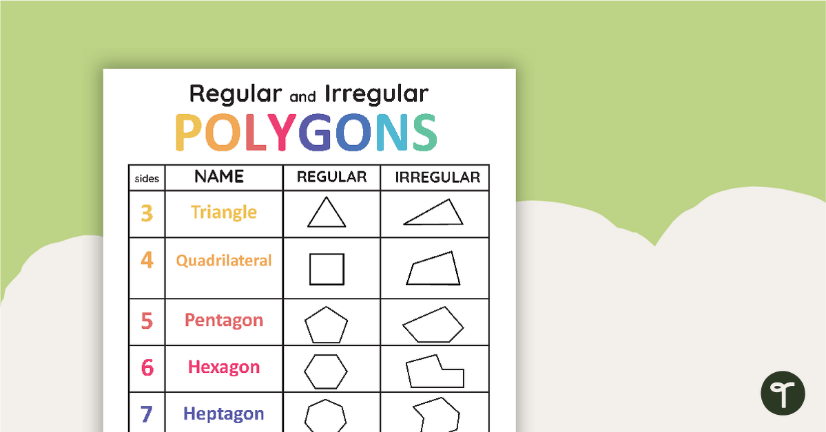
Polygons are often named based on how many sides they have.

Triangle

A polygon with 3 sides.

Example:

Equilateral triangle.


Quadrilateral

A polygon with 4 sides.

Examples include squares and rectangles.


Pentagon

A polygon with 5 sides.

Example:

The shape of many national buildings and logos.


Hexagon

A polygon with 6 sides.

Example:

Honeycomb cells created by bees.


Heptagon

A polygon with 7 sides.


Octagon

A polygon with 8 sides.

Example:

Stop traffic sign.


Nonagon

A polygon with 9 sides.


Decagon

A polygon with 10 sides.


Regular Polygons

A regular polygon has:

  • All sides equal
  • All angles equal

Examples:

  • Equilateral triangle
  • Square
  • Regular pentagon
  • Regular hexagon

Regular polygons are highly symmetrical.


Irregular Polygons

An irregular polygon does not have equal sides or equal angles.

Example:

A quadrilateral with unequal sides.


Convex Polygons

A polygon is convex if all interior angles are less than 180°.

Properties:

  • All diagonals lie inside the polygon.
  • The shape bulges outward.

Most common polygons are convex.


Concave Polygons

A concave polygon has at least one interior angle greater than 180°.

Properties:

  • Some diagonals lie outside the polygon.
  • The shape has an inward indentation.

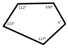
Interior Angles of Polygons

The sum of the interior angles of a polygon depends on the number of sides.

Formula:

[
(n-2) \times 180^\circ
]

Where:

(n) = number of sides.

Example:

For a pentagon:

[
(5-2)\times180 = 540^\circ
]


Interior Angle of Regular Polygon

In a regular polygon, all interior angles are equal.

Formula:

[
\frac{(n-2) \times 180}{n}
]

Example:

Hexagon:

[
\frac{(6-2)\times180}{6} = 120^\circ
]


Exterior Angles of Polygons

Exterior angles are formed when a side of the polygon is extended.

The sum of all exterior angles of any polygon is always:

[
360^\circ
]

This rule applies regardless of the number of sides.


Number of Diagonals in a Polygon

The number of diagonals in a polygon is given by the formula:

[
\frac{n(n-3)}{2}
]

Example:

For a hexagon:

[
\frac{6(6-3)}{2} = 9
]

So a hexagon has 9 diagonals.


Area of Polygons

Different polygons have different area formulas.


Area of a Triangle

[
A = \frac{1}{2}bh
]


Area of a Square

[
A = s^2
]

Where (s) is side length.


Area of a Rectangle

[
A = length \times width
]


Area of a Regular Polygon

Formula:

[
A = \frac{1}{2} ap
]

Where:

  • (a) = apothem
  • (p) = perimeter

Apothem

The apothem is the perpendicular distance from the center of a regular polygon to one of its sides.

It helps calculate the area of regular polygons.


Perimeter of Polygons

The perimeter of a polygon is the total length of its sides.

Example:

If a pentagon has sides:

5, 5, 5, 5, 5

Perimeter:

[
25
]


Symmetry in Polygons

Regular polygons have symmetrical properties.

Example:

A square has:

  • 4 lines of symmetry
  • rotational symmetry

Regular polygons have symmetry equal to the number of sides.


Tessellations

Polygons can be used to tile a plane without gaps.

This is called tessellation.

Examples:

  • Squares
  • Equilateral triangles
  • Regular hexagons

These shapes can cover surfaces completely.


Polygons in Coordinate Geometry

Polygons can be represented using coordinates.

Example:

Vertices:

[
(1,2), (4,2), (4,5), (1,5)
]

These points form a rectangle.

Coordinate geometry allows calculation of:

  • distance
  • slopes
  • area

Applications of Polygons

Polygons are used extensively in real-world applications.


Architecture

Buildings and floor plans often use polygonal shapes.


Engineering

Engineers use polygons to design structures and mechanical components.


Computer Graphics

Polygons form the basis of 3D models and digital images.

Example:

Video games use polygons to create objects.


Cartography

Maps use polygons to represent regions and boundaries.


Art and Design

Polygons are used in patterns, mosaics, and decorative designs.


Polygons in Nature

Many natural structures resemble polygons.

Examples include:

  • honeycombs
  • crystal shapes
  • turtle shells

Hexagonal shapes in honeycombs maximize space efficiency.


Historical Development of Polygon Geometry

Ancient mathematicians studied polygons extensively.

Greek mathematician Euclid analyzed properties of regular polygons.

Later mathematicians expanded polygon geometry through trigonometry and analytic geometry.

Today, polygons remain essential in both pure mathematics and applied sciences.


Polygons in Advanced Mathematics

Polygons are important in advanced topics such as:

  • computational geometry
  • topology
  • fractal geometry
  • polygon triangulation

These concepts help analyze complex shapes and algorithms.


Importance of Polygons

Polygons are important because they:

  • form the basis of geometric shapes
  • help calculate areas and perimeters
  • appear in architecture and engineering
  • form the foundation of computer graphics

Understanding polygons helps build knowledge of geometry and spatial reasoning.


Conclusion

Polygons are fundamental geometric shapes formed by straight line segments connected to create closed figures. They include a wide range of shapes such as triangles, quadrilaterals, pentagons, hexagons, and many others. By studying polygons, mathematicians gain insight into geometric relationships, symmetry, angle measurements, and area calculations.

Polygons also play a crucial role in many practical applications including architecture, engineering, computer graphics, and design. Their simple yet powerful structure allows them to represent both basic shapes and complex models in mathematics and technology.

Through the study of polygons, students develop essential geometric skills that support further learning in trigonometry, coordinate geometry, and advanced mathematical analysis.


Tags

Circles in Mathematics

Image
Image
Image
Image

Introduction to Circles

A circle is one of the most fundamental and widely studied shapes in geometry. It appears frequently in mathematics, science, engineering, architecture, astronomy, and everyday life. From wheels and coins to planetary orbits and waves, circles play a crucial role in understanding shapes and motion.

In geometry, a circle represents a perfectly symmetrical figure where every point on its boundary is at the same distance from a central point. This constant distance defines the size of the circle and is known as the radius.

Circles have fascinated mathematicians for thousands of years. Ancient civilizations studied circles to understand astronomical movements, construct buildings, and measure land. Today, circles are used extensively in modern technology, computer graphics, physics, and engineering.

The study of circles includes many important concepts such as radius, diameter, chords, arcs, sectors, tangents, and angles. These concepts help us understand the geometric properties of circular shapes and their applications in both theoretical and practical contexts.


Definition of a Circle

A circle is defined as the set of all points in a plane that are at a fixed distance from a given point.

The fixed point is called the center of the circle.

The fixed distance is called the radius.

Mathematically:

A circle with center (O) and radius (r) consists of all points (P) such that:

[
OP = r
]

This means every point on the circle lies exactly the same distance from the center.


Basic Components of a Circle

A circle contains several important elements that help describe its geometry.


Center

The center of a circle is the point located exactly in the middle of the circle.

It is usually represented by the letter O.

All points on the circumference of the circle are equidistant from the center.


Radius

The radius is the distance from the center of the circle to any point on its boundary.

Symbol:

[
r
]

Example:

If the radius of a circle is 5 cm, every point on the circle is exactly 5 cm away from the center.


Diameter

The diameter is the longest chord of the circle and passes through the center.

It connects two points on the circle and passes directly through the center.

Formula:

[
d = 2r
]

Where:

  • (d) = diameter
  • (r) = radius

Circumference

The circumference is the distance around the circle.

Formula:

[
C = 2\pi r
]

Or

[
C = \pi d
]

Where:

(\pi) is approximately 3.14159.


Area of a Circle

The area of a circle represents the space enclosed inside the circle.

Formula:

[
A = \pi r^2
]

Example:

If radius = 7 cm

[
A = \pi \times 7^2
]

[
A = 49\pi
]


Chord

A chord is a line segment that connects two points on the circle.

The diameter is the longest chord in a circle.

Properties:

  • Every diameter is a chord.
  • Not every chord is a diameter.

Arc

An arc is a part of the circumference of the circle.

There are two types of arcs:

Minor Arc

The smaller arc between two points.

Major Arc

The larger arc between two points.


Sector

A sector is a region bounded by two radii and an arc.

Example:

A slice of pizza is an example of a sector.

Area formula:

[
A = \frac{\theta}{360} \times \pi r^2
]

Where (\theta) is the central angle.


Segment

A segment is the region between a chord and the arc.

Segments can be minor or major depending on the size.


Tangent

A tangent is a line that touches the circle at exactly one point.

Properties:

  • Tangent touches circle at one point.
  • Tangent is perpendicular to the radius at the point of contact.

Secant

A secant is a line that intersects a circle at two points.

Unlike a tangent, it passes through the circle.


Concentric Circles

Two or more circles with the same center but different radii are called concentric circles.

Example:

Ripples formed when a stone drops in water.


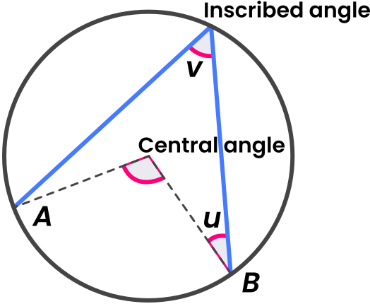
Central Angle

A central angle is an angle formed by two radii of the circle.

The vertex of the angle is at the center.

The measure of the arc equals the central angle.

Example:

If central angle = 60°

Arc measure = 60°.


Inscribed Angle

An inscribed angle is an angle whose vertex lies on the circle and whose sides contain chords.

The measure of an inscribed angle equals half the measure of the intercepted arc.

Formula:

[
\angle = \frac{1}{2} arc
]


Theorems Related to Circles

Many important theorems describe relationships between parts of circles.


Angle in a Semicircle

The angle formed in a semicircle is always a right angle.

This theorem is widely used in geometry.


Tangent Radius Theorem

A tangent is perpendicular to the radius at the point of contact.


Equal Chords Theorem

Equal chords are equidistant from the center of the circle.


Perpendicular Bisector of a Chord

The perpendicular bisector of a chord passes through the center.


Intersecting Chords Theorem

If two chords intersect inside a circle:

[
a \times b = c \times d
]


Tangent-Secant Theorem

If a tangent and a secant are drawn from a point outside the circle:

[
t^2 = external \times whole
]


Equations of Circles in Coordinate Geometry

In coordinate geometry, circles are represented by equations.

Standard form:

[
(x-h)^2 + (y-k)^2 = r^2
]

Where:

  • (h,k) = center
  • (r) = radius

Example:

[
(x-2)^2 + (y-3)^2 = 25
]

Center = (2,3)
Radius = 5


General Equation of a Circle

General form:

[
x^2 + y^2 + Dx + Ey + F = 0
]

This equation can be converted to standard form.


Length of an Arc

Arc length formula:

[
L = \frac{\theta}{360} \times 2\pi r
]

Where:

(\theta) = central angle.


Area of a Sector

[
A = \frac{\theta}{360} \times \pi r^2
]


Circles in Trigonometry

The unit circle is important in trigonometry.

It has radius = 1.

Used to define:

  • sine
  • cosine
  • tangent

Circles in Real Life

Circles appear everywhere in everyday life.

Examples include:

  • wheels
  • coins
  • clocks
  • plates
  • gears
  • planets
  • lenses

Circles in Engineering

Engineers use circular designs for:

  • rotating machinery
  • wheels
  • gears
  • turbines

Circular shapes distribute forces evenly.


Circles in Astronomy

Planetary orbits are often studied using circular and elliptical models.

Circular motion is important in physics and astronomy.


Circles in Architecture

Architectural structures such as domes and arches often use circular shapes.

Examples:

  • stadium roofs
  • bridges
  • arches

Historical Development of Circle Geometry

The study of circles dates back to ancient civilizations.

Egyptians and Babylonians studied circular measurements.

Greek mathematicians developed systematic geometry of circles.

One of the most famous discoveries related to circles is the constant π (pi).

Pi represents the ratio between circumference and diameter.


Importance of Circles in Mathematics

Circles are essential because they:

  • represent symmetry
  • connect geometry with trigonometry
  • appear in calculus
  • model circular motion
  • describe waves and rotations

They provide a bridge between algebra, geometry, and physics.


Circles in Calculus

Circles appear in calculus when studying curves and motion.

Example:

Parametric equations of a circle:

[
x = r\cos\theta
]

[
y = r\sin\theta
]

These equations describe circular motion.


Advanced Concepts Related to Circles

Advanced mathematics studies concepts such as:

  • cyclic quadrilaterals
  • circle inversion
  • complex numbers and the unit circle
  • circular functions

These topics extend the study of circles into higher mathematics.


Conclusion

Circles are one of the most important and elegant shapes in mathematics. Defined as the set of all points equidistant from a central point, circles possess unique properties that make them essential in geometry, trigonometry, and many scientific disciplines.

The study of circles includes various components such as radius, diameter, chords, arcs, sectors, tangents, and angles. These elements help mathematicians understand relationships within circular shapes and solve geometric problems.

Beyond theoretical mathematics, circles appear extensively in real-world applications, including engineering designs, architectural structures, astronomy, and mechanical systems. Their symmetry and efficiency make them fundamental in both natural phenomena and human-made technologies.

Understanding circles provides a foundation for advanced mathematical concepts and highlights the deep connections between geometry, algebra, and science.


Tags

Triangles and Quadrilaterals in Mathematics

Image
Image
Image
Image

Introduction to Triangles

Triangles are among the most fundamental shapes studied in geometry. A triangle is a polygon that has three sides, three vertices, and three angles. Despite its simple structure, the triangle possesses a rich set of properties and plays a central role in many areas of mathematics, especially in geometry and trigonometry.

Triangles appear in many natural and human-made structures. For example, bridges, roofs, and frameworks often use triangular designs because triangles provide structural stability. In mathematics, triangles help establish important geometric relationships such as angle sums, congruence, similarity, and trigonometric functions.

The study of triangles allows mathematicians to understand spatial relationships, solve measurement problems, and analyze shapes in both two-dimensional and three-dimensional spaces.


Definition of a Triangle

A triangle is a closed polygon formed by three line segments connecting three distinct points.

If the vertices are named A, B, and C, the triangle is written as:

[
\triangle ABC
]

The three sides are:

AB, BC, and CA

The three angles are:

∠A, ∠B, and ∠C


Basic Properties of Triangles

Triangles have several important properties.

Number of Sides

A triangle always has three sides.


Number of Angles

A triangle always has three angles.


Sum of Interior Angles

The sum of interior angles of a triangle is:

[
180^\circ
]

Example:

If two angles are 50° and 60°, the third angle is:

[
180 – (50 + 60) = 70^\circ
]


Exterior Angle Property

An exterior angle of a triangle equals the sum of the two opposite interior angles.

Example:

If two interior angles are 40° and 60°, the exterior angle is:

[
100^\circ
]


Classification of Triangles Based on Sides

Triangles can be categorized according to their side lengths.


Equilateral Triangle

An equilateral triangle has all three sides equal.

Properties:

  • All sides equal
  • All angles equal
  • Each angle = 60°

Example:

Triangle ABC with sides:

AB = BC = CA


Isosceles Triangle

An isosceles triangle has two equal sides.

Properties:

  • Two sides equal
  • Base angles equal

Example:

AB = AC

Angles at B and C are equal.


Scalene Triangle

A scalene triangle has all sides different.

Properties:

  • No equal sides
  • No equal angles

Example:

Triangle with sides:

3, 4, 5


Classification Based on Angles

Triangles can also be classified by their angles.


Acute Triangle

All three angles are less than 90°.

Example:

45°, 60°, 75°


Right Triangle

One angle equals 90°.

Example:

3–4–5 triangle.

Right triangles are essential in trigonometry.


Obtuse Triangle

One angle is greater than 90°.

Example:

120°, 30°, 30°


Important Elements of a Triangle

Triangles include several special line segments.


Median

A median connects a vertex to the midpoint of the opposite side.

All three medians intersect at a point called the centroid.


Altitude

An altitude is a perpendicular line from a vertex to the opposite side.

The intersection of altitudes is called the orthocenter.


Angle Bisector

An angle bisector divides an angle into two equal parts.

The intersection of angle bisectors is called the incenter.


Perpendicular Bisector

A perpendicular bisector divides a side into two equal parts at 90°.

The intersection point is called the circumcenter.


Congruence of Triangles

Two triangles are congruent if they are exactly the same in shape and size.

Congruence rules include:

SSS (Side-Side-Side)

Three sides equal.

SAS (Side-Angle-Side)

Two sides and included angle equal.

ASA (Angle-Side-Angle)

Two angles and included side equal.

RHS (Right angle-Hypotenuse-Side)

Used for right triangles.


Similarity of Triangles

Two triangles are similar if they have the same shape but different sizes.

Similarity rules include:

AA (Angle-Angle)

Two angles equal.

SAS Similarity

Two sides proportional with included angle equal.

SSS Similarity

Three sides proportional.


Area of a Triangle

Area formula:

[
Area = \frac{1}{2} \times base \times height
]

Another formula using Heron’s formula:

[
Area = \sqrt{s(s-a)(s-b)(s-c)}
]

Where:

[
s = \frac{a+b+c}{2}
]


Pythagorean Theorem

In right triangles:

[
a^2 + b^2 = c^2
]

Where:

c = hypotenuse

This theorem is fundamental in geometry.


Applications of Triangles

Triangles are used in:

  • bridge construction
  • trigonometry
  • navigation
  • surveying
  • architecture

Their structural strength makes them important in engineering.


Quadrilaterals

Image
Image
Image

Definition of Quadrilateral

A quadrilateral is a polygon with four sides, four vertices, and four angles.

Example:

Quadrilateral ABCD


Properties of Quadrilaterals

Important properties include:

  • Four sides
  • Four vertices
  • Four angles
  • Two diagonals

The sum of interior angles equals:

[
360^\circ
]


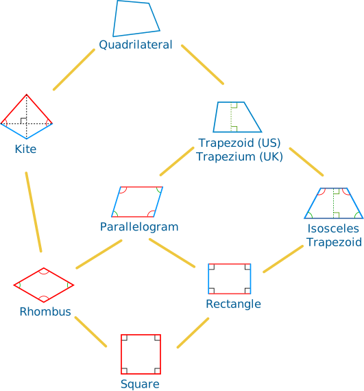
Types of Quadrilaterals

Quadrilaterals are classified based on side lengths and angle properties.


Parallelogram

A parallelogram is a quadrilateral in which opposite sides are parallel.

Properties:

  • Opposite sides equal
  • Opposite angles equal
  • Diagonals bisect each other

Area:

[
Area = base \times height
]


Rectangle

A rectangle is a parallelogram with four right angles.

Properties:

  • Opposite sides equal
  • All angles = 90°
  • Diagonals equal

Area:

[
Area = length \times width
]


Square

A square is a special rectangle with all sides equal.

Properties:

  • All sides equal
  • All angles = 90°
  • Diagonals equal and perpendicular

Area:

[
Area = side^2
]


Rhombus

A rhombus has all sides equal but angles are not necessarily 90°.

Properties:

  • All sides equal
  • Opposite angles equal
  • Diagonals perpendicular

Area:

[
Area = \frac{1}{2} d_1 d_2
]


Trapezium (Trapezoid)

A trapezium has one pair of parallel sides.

Properties:

  • Two sides parallel
  • Other sides non-parallel

Area:

[
Area = \frac{1}{2}(a+b)h
]


Kite

A kite has two pairs of adjacent equal sides.

Properties:

  • Diagonals perpendicular
  • One diagonal bisects the other

Diagonals of Quadrilaterals

A diagonal connects opposite vertices.

Quadrilaterals always have two diagonals.

Diagonals divide quadrilaterals into triangles.


Angle Properties of Quadrilaterals

The sum of interior angles is always:

[
360^\circ
]

Example:

If three angles are:

80°, 100°, 120°

Fourth angle:

[
360 – 300 = 60^\circ
]


Area Formulas of Quadrilaterals

Different quadrilaterals have different area formulas.

Rectangle:

[
A = lw
]

Square:

[
A = a^2
]

Parallelogram:

[
A = bh
]

Rhombus:

[
A = \frac{1}{2} d_1 d_2
]

Trapezium:

[
A = \frac{1}{2}(a+b)h
]


Applications of Quadrilaterals

Quadrilaterals appear in:

  • floor designs
  • building structures
  • road layouts
  • computer graphics
  • tiling patterns

Many architectural designs rely heavily on quadrilateral shapes.


Relationship Between Triangles and Quadrilaterals

Quadrilaterals can be divided into two triangles by drawing a diagonal.

This property helps calculate areas and analyze geometric relationships.

Triangles and quadrilaterals together form the basis for studying polygons.


Historical Development

Ancient civilizations studied triangles and quadrilaterals for land measurement and construction.

Greek mathematicians such as Euclid developed systematic theories of geometry.

Later mathematicians expanded these concepts in coordinate geometry and analytic geometry.

Today, triangles and quadrilaterals remain essential elements of geometric study.


Importance in Mathematics

Triangles and quadrilaterals are crucial because they:

  • form the basis of polygon geometry
  • support trigonometry
  • help analyze shapes and areas
  • appear in engineering structures
  • assist in computer graphics and design

These shapes provide the foundation for understanding more complex geometric figures.


Conclusion

Triangles and quadrilaterals are fundamental geometric shapes that play an essential role in mathematics and real-world applications. A triangle, with its three sides and angles, provides the basis for many geometric theorems and trigonometric relationships. Quadrilaterals, with their four sides and angles, include a variety of shapes such as squares, rectangles, parallelograms, rhombuses, trapeziums, and kites.

Together, these shapes help mathematicians analyze space, measure areas, understand symmetry, and solve complex geometric problems. From architectural structures and engineering designs to computer graphics and scientific modeling, triangles and quadrilaterals remain among the most important shapes studied in geometry.

Mastering these concepts builds a strong foundation for advanced topics such as trigonometry, coordinate geometry, and three-dimensional geometry.


Tags

Points, Lines, and Angles

Image
Image
Image
Image

Introduction to Points, Lines, and Angles

Points, lines, and angles are among the most fundamental concepts in geometry. Geometry itself is a branch of mathematics that deals with shapes, sizes, positions of figures, and the properties of space. Every geometric figure—from simple triangles to complex three-dimensional structures—begins with these basic elements.

Understanding points, lines, and angles provides the foundation for studying more advanced mathematical topics such as polygons, circles, coordinate geometry, trigonometry, and calculus. These concepts also have real-world applications in architecture, engineering, physics, navigation, and computer graphics.

A point represents a specific location in space, a line represents a straight path extending infinitely in both directions, and an angle represents the amount of rotation between two intersecting lines or rays.

These basic elements are the building blocks from which all geometric figures are constructed.


Points in Geometry

Definition of a Point

A point is the most basic object in geometry. It represents an exact location in space but has no size, length, width, or thickness.

In geometry, points are usually represented by capital letters such as:

A, B, C, D

A point is often shown as a small dot on a diagram.

Example:

Point A

A point only indicates position, not dimension.


Properties of a Point

Important characteristics of points include:

  • A point has no dimension
  • It represents a location
  • It cannot be measured
  • It is usually named with capital letters

Points serve as references for defining other geometric objects.


Points in Coordinate Geometry

In coordinate geometry, points are represented using coordinates.

Example:

[
(x, y)
]

This indicates a point on the coordinate plane.

Example:

[
(3,4)
]

This means the point lies 3 units along the x-axis and 4 units along the y-axis.

In three-dimensional space, a point is represented as:

[
(x,y,z)
]


Distance Between Two Points

The distance between two points in a coordinate plane is calculated using the distance formula.

For two points:

[
(x_1,y_1) \quad and \quad (x_2,y_2)
]

Distance:

[
d=\sqrt{(x_2-x_1)^2+(y_2-y_1)^2}
]

This formula is derived from the Pythagorean theorem.


Midpoint Between Two Points

The midpoint of a line segment joining two points is:

[
M\left(\frac{x_1+x_2}{2},\frac{y_1+y_2}{2}\right)
]

The midpoint divides the segment into two equal parts.


Lines in Geometry

Definition of a Line

A line is a straight path that extends infinitely in both directions.

A line has length but no thickness.

Lines are usually named using:

  • two points on the line
  • a lowercase letter

Example:

Line AB

Written as:

[
\overleftrightarrow{AB}
]


Properties of Lines

Important properties include:

  • A line extends infinitely
  • It has no endpoints
  • It has only one dimension: length
  • It contains infinitely many points

Types of Lines

Geometry includes several types of lines.


Line Segment

A line segment is a part of a line that has two endpoints.

Example:

Segment AB

Notation:

[
\overline{AB}
]

Unlike a line, a line segment has a fixed length.


Ray

A ray is a part of a line that begins at one point and extends infinitely in one direction.

Example:

Ray AB

Notation:

[
\overrightarrow{AB}
]

Here A is the endpoint.


Parallel Lines

Two lines are parallel if they never intersect.

Symbol:

[
l_1 \parallel l_2
]

Properties:

  • Always maintain equal distance
  • Never meet

Example:

Railroad tracks.


Perpendicular Lines

Two lines are perpendicular if they intersect at a right angle.

Symbol:

[
l_1 \perp l_2
]

The angle between them is:

[
90^\circ
]


Intersecting Lines

When two lines cross each other at a point, they are intersecting lines.

Example:

The letter “X”.


Skew Lines

In three-dimensional space, skew lines do not intersect and are not parallel.

They lie in different planes.


Angles in Geometry

Definition of an Angle

An angle is formed when two rays share a common endpoint.

The common endpoint is called the vertex.

The rays are called arms of the angle.

Example:

Angle ABC

Where B is the vertex.

Notation:

[
\angle ABC
]


Measurement of Angles

Angles are measured in degrees.

A full rotation equals:

[
360^\circ
]

Other units include radians used in advanced mathematics.


Types of Angles

Angles are classified according to their measure.


Acute Angle

An angle less than 90°.

Example:

[
45^\circ
]


Right Angle

Exactly 90°.

Often marked with a small square in diagrams.


Obtuse Angle

Greater than 90° but less than 180°.

Example:

[
120^\circ
]


Straight Angle

Exactly 180°.

Forms a straight line.


Reflex Angle

Greater than 180° but less than 360°.

Example:

[
240^\circ
]


Complete Angle

A full rotation.

[
360^\circ
]


Adjacent Angles

Adjacent angles share a common vertex and a common side but do not overlap.

Example:

Angles forming a corner.


Complementary Angles

Two angles whose sum equals:

[
90^\circ
]

Example:

[
30^\circ + 60^\circ
]


Supplementary Angles

Two angles whose sum equals:

[
180^\circ
]

Example:

[
120^\circ + 60^\circ
]


Vertical Angles

When two lines intersect, opposite angles are called vertical angles.

Vertical angles are always equal.


Linear Pair

A pair of adjacent angles that sum to:

[
180^\circ
]

They form a straight line.


Angles Formed by Parallel Lines

When a transversal intersects two parallel lines, several angles are formed.

Important types include:

  • Corresponding angles
  • Alternate interior angles
  • Alternate exterior angles
  • Consecutive interior angles

Corresponding Angles

These angles occupy similar positions at intersections.

They are equal when lines are parallel.


Alternate Interior Angles

Located inside the parallel lines on opposite sides of the transversal.

They are equal.


Alternate Exterior Angles

Located outside the parallel lines on opposite sides of the transversal.

They are also equal.


Consecutive Interior Angles

Also called co-interior angles.

Their sum equals:

[
180^\circ
]


Angle Bisector

An angle bisector divides an angle into two equal parts.

Example:

If angle = 60°

Each part becomes:

[
30^\circ
]


Relationship Between Points, Lines, and Angles

Points define lines.

Lines form angles.

Angles create shapes such as triangles and polygons.

For example:

  • Two points define a line
  • Two lines intersect to form angles
  • Three points define a triangle

Applications in Real Life

Points, lines, and angles appear everywhere in the real world.


Architecture

Architects use angles and lines to design buildings.


Engineering

Engineers use geometry to construct bridges, machines, and structures.


Navigation

Angles help determine direction and distance.


Computer Graphics

Graphics systems use geometric principles to render shapes.


Astronomy

Astronomers measure angles to determine distances between celestial bodies.


Points, Lines, and Angles in Coordinate Geometry

In coordinate geometry, lines are represented using equations.

Example:

[
y = mx + c
]

Where:

  • (m) = slope
  • (c) = intercept

Angles between lines can be calculated using slopes.

Formula:

[
\tan \theta = \frac{m_1 – m_2}{1 + m_1m_2}
]


Historical Development

Geometry was studied extensively by ancient civilizations.

Egyptians used geometric principles for land measurement.

Greek mathematician Euclid organized geometry into a logical system in his famous work Elements.

Euclidean geometry established the fundamental definitions of points, lines, and angles.

These ideas remain central to modern mathematics.


Importance in Mathematics

Points, lines, and angles are essential because they:

  • form the basis of geometry
  • define shapes and figures
  • allow measurement of space
  • support advanced mathematics such as trigonometry and calculus

Understanding these concepts is necessary for studying higher mathematics.


Conclusion

Points, lines, and angles are the fundamental building blocks of geometry and spatial understanding. A point represents a position, a line represents a continuous path, and an angle represents the relationship between two intersecting lines. Together, these elements form the basis of geometric figures and structures used in mathematics and real-world applications.

From simple geometric constructions to complex architectural designs and scientific measurements, these concepts play a vital role in understanding space and structure. By mastering points, lines, and angles, students gain a strong foundation for exploring advanced topics such as polygons, trigonometry, coordinate geometry, and three-dimensional geometry.

Their simplicity combined with their wide-ranging applications makes them one of the most essential topics in mathematics.


Tags

Logarithms in Mathematics

Image
Image
Image
Image

Introduction to Logarithms

Logarithms are one of the most important concepts in mathematics, especially in algebra, calculus, and many scientific fields. They provide a powerful way to solve exponential equations, analyze growth and decay processes, and simplify complex mathematical calculations.

A logarithm is essentially the inverse operation of exponentiation. If exponentiation asks the question, “How many times should a base be multiplied by itself to produce a number?”, logarithms answer the reverse question: “To what power must a base be raised to obtain a given number?”

For example, consider the exponential expression:

[
2^3 = 8
]

This means that 2 multiplied by itself three times equals 8.

The equivalent logarithmic form is:

[
\log_2 8 = 3
]

This reads as: “The logarithm of 8 with base 2 is 3.” In other words, 2 must be raised to the power of 3 to obtain 8.

Logarithms are used in a wide variety of fields including physics, computer science, engineering, statistics, economics, chemistry, and information theory. They simplify calculations involving very large or very small numbers and are essential for analyzing exponential growth or decay.


Definition of Logarithm

A logarithm is defined as the exponent to which a base must be raised to produce a given number.

General form:

[
\log_b a = c
]

This means:

[
b^c = a
]

Where:

  • (b) = base
  • (a) = argument (the number inside the logarithm)
  • (c) = logarithmic value (the exponent)

Example:

[
\log_3 27 = 3
]

Because:

[
3^3 = 27
]


Historical Background of Logarithms

Logarithms were developed in the early 17th century to simplify complex arithmetic calculations.

The Scottish mathematician John Napier introduced the concept of logarithms around 1614. His goal was to make multiplication and division easier by converting them into addition and subtraction.

Later, mathematician Henry Briggs refined Napier’s work and introduced the base-10 logarithm, which became widely used in scientific calculations.

Before the invention of calculators and computers, logarithmic tables were essential tools for scientists, engineers, and astronomers.


Relationship Between Exponents and Logarithms

Logarithms and exponents are closely related.

Exponential form:

[
b^x = y
]

Logarithmic form:

[
\log_b y = x
]

Example:

[
10^4 = 10000
]

Equivalent logarithmic form:

[
\log_{10} 10000 = 4
]

Understanding this relationship is essential for solving exponential equations.


Types of Logarithms

Several types of logarithms are commonly used in mathematics and science.


Common Logarithm

A common logarithm has base 10.

Notation:

[
\log x
]

Example:

[
\log 100 = 2
]

Because:

[
10^2 = 100
]

Common logarithms are widely used in engineering and scientific calculations.


Natural Logarithm

A natural logarithm has base (e), where (e) is an important mathematical constant approximately equal to 2.718.

Notation:

[
\ln x
]

Example:

[
\ln e = 1
]

Because:

[
e^1 = e
]

Natural logarithms appear frequently in calculus and exponential growth models.


Binary Logarithm

A binary logarithm has base 2.

Notation:

[
\log_2 x
]

Example:

[
\log_2 16 = 4
]

Binary logarithms are important in computer science, especially in analyzing algorithm complexity.


Logarithmic Functions

A logarithmic function has the form:

[
f(x) = \log_b x
]

Where:

  • (b > 0)
  • (b \neq 1)

Properties:

  • Domain: (x > 0)
  • Range: all real numbers

The logarithmic function is the inverse of the exponential function.


Graph of Logarithmic Functions

Logarithmic functions have distinctive graphs.

Key characteristics include:

  • Defined only for positive values of (x)
  • Increasing slowly
  • Passing through point (1,0)

Example:

[
\log_b 1 = 0
]

Graphically, logarithmic curves increase but flatten gradually.


Properties of Logarithms

Logarithms follow several important algebraic rules.


Product Rule

The logarithm of a product equals the sum of logarithms.

[
\log_b (xy) = \log_b x + \log_b y
]

Example:

[
\log(1000 \times 100) = \log 1000 + \log 100
]


Quotient Rule

The logarithm of a quotient equals the difference of logarithms.

[
\log_b \frac{x}{y} = \log_b x – \log_b y
]


Power Rule

The logarithm of a power equals the exponent multiplied by the logarithm.

[
\log_b (x^n) = n \log_b x
]

Example:

[
\log(100^2) = 2 \log 100
]


Logarithm of 1

[
\log_b 1 = 0
]

Because:

[
b^0 = 1
]


Logarithm of the Base

[
\log_b b = 1
]

Because:

[
b^1 = b
]


Change of Base Formula

Logarithms can be converted from one base to another.

Formula:

[
\log_b a = \frac{\log_c a}{\log_c b}
]

Commonly used with base 10 or base (e).

Example:

[
\log_2 8 = \frac{\log 8}{\log 2}
]


Solving Logarithmic Equations

Example:

[
\log_2 x = 5
]

Rewrite as exponential equation:

[
2^5 = x
]

[
x = 32
]


Example with two logarithms:

[
\log(x) + \log(2) = 3
]

Using product rule:

[
\log(2x) = 3
]

Convert to exponential form:

[
10^3 = 2x
]

[
x = 500
]


Logarithmic Inequalities

Logarithmic inequalities follow similar rules as logarithmic equations.

Example:

[
\log x > 2
]

Convert to exponential form:

[
x > 100
]

But domain restriction applies:

[
x > 0
]


Applications of Logarithms

Logarithms are widely used in many real-world applications.


Scientific Measurements

Logarithmic scales are used to measure quantities that vary over large ranges.

Examples include:

  • pH scale in chemistry
  • Richter scale for earthquakes
  • decibel scale for sound intensity

Computer Science

Logarithms are essential in analyzing algorithms.

Example:

Binary search algorithm complexity:

[
O(\log n)
]


Finance

Logarithms help analyze compound interest and continuous growth.

Example:

[
A = Pe^{rt}
]

Solving for time often requires logarithms.


Physics

Logarithms appear in equations describing:

  • radioactive decay
  • wave intensity
  • entropy

Information Theory

Logarithms measure information content.

Example:

Shannon entropy uses base-2 logarithms.


Logarithmic Scales

Logarithmic scales compress large ranges into manageable numbers.

Example:

Richter scale.

An earthquake measuring 7 is ten times stronger than one measuring 6.


Logarithms in Calculus

Logarithmic functions are essential in calculus.

Derivative:

[
\frac{d}{dx}(\ln x) = \frac{1}{x}
]

Integral:

[
\int \frac{1}{x} dx = \ln |x| + C
]

Logarithms simplify many integration and differentiation problems.


Logarithmic Growth

Logarithmic growth increases slowly over time.

Example:

Population growth slowing after saturation.


Logarithmic vs Exponential Growth

Exponential growth increases rapidly.

Logarithmic growth increases slowly.

Example comparison:

[
y = e^x
]

vs

[
y = \ln x
]

Exponential functions grow much faster.


Logarithms in Data Science

Logarithmic transformations are used to normalize skewed data.

Example:

Income distributions often use log transformations.


Importance of Logarithms

Logarithms are crucial because they:

  • simplify multiplication and division
  • solve exponential equations
  • analyze exponential growth
  • compress large numerical ranges
  • appear in advanced mathematics and science

They form an essential part of mathematical analysis and modeling.


Conclusion

Logarithms are powerful mathematical tools that allow us to work with exponential relationships and simplify complex calculations. By transforming multiplication into addition and exponentiation into multiplication, logarithms make it easier to solve equations, analyze growth processes, and handle large numerical ranges.

From scientific measurement scales and computer algorithms to financial models and calculus, logarithms play a central role in both theoretical mathematics and practical applications. Their deep connection with exponential functions makes them indispensable for understanding natural phenomena, technological systems, and mathematical structures.

Mastering logarithms provides a strong foundation for advanced mathematics, including calculus, statistics, and scientific modeling, making them one of the most important concepts in mathematical study.


Tags

Sequences and Series in Mathematics

Image
Image
Image
Image

Introduction to Sequences and Series

In mathematics, sequences and series are fundamental concepts that describe ordered patterns of numbers and the sum of those patterns. These ideas play a central role in algebra, calculus, number theory, statistics, and mathematical analysis. They also appear frequently in scientific fields such as physics, economics, computer science, engineering, and finance.

A sequence is an ordered list of numbers that follow a specific rule or pattern. Each number in the sequence is called a term, and the position of the term usually determines its value.

For example:

[
2, 4, 6, 8, 10
]

This is a sequence of even numbers increasing by 2.

A series, on the other hand, is the sum of the terms of a sequence.

For example:

[
2 + 4 + 6 + 8 + 10
]

This represents a series derived from the sequence above.

Sequences and series are powerful tools because they allow mathematicians to analyze patterns, approximate values, solve equations, and model real-world phenomena.


Definition of Sequence

A sequence is an ordered list of numbers written in a specific order according to a defined rule.

A sequence is typically written as:

[
a_1, a_2, a_3, a_4, …
]

Where:

  • (a_1) = first term
  • (a_2) = second term
  • (a_n) = nth term

Example sequence:

[
1, 3, 5, 7, 9
]

Here:

  • (a_1 = 1)
  • (a_2 = 3)
  • (a_3 = 5)

Each term follows the rule:

[
a_n = 2n – 1
]


Notation for Sequences

Sequences are commonly written using notation:

[
{a_n}
]

Where (n) represents the position of the term.

Example:

[
a_n = n^2
]

Sequence becomes:

[
1, 4, 9, 16, 25, …
]


Types of Sequences

There are many types of sequences used in mathematics.


Finite Sequence

A finite sequence contains a limited number of terms.

Example:

[
2, 4, 6, 8
]

Only four terms exist.


Infinite Sequence

An infinite sequence continues indefinitely.

Example:

[
1, 2, 3, 4, 5, …
]

The sequence continues forever.


Arithmetic Sequence

An arithmetic sequence is a sequence in which the difference between consecutive terms is constant.

This constant difference is called the common difference.

Example:

[
5, 8, 11, 14, 17
]

Common difference:

[
d = 3
]

General formula:

[
a_n = a_1 + (n-1)d
]

Example:

First term = 5
Common difference = 3

[
a_n = 5 + (n-1)3
]


Example of Arithmetic Sequence

Sequence:

[
3, 7, 11, 15, 19
]

First term:

[
a_1 = 3
]

Common difference:

[
d = 4
]

10th term:

[
a_{10} = 3 + (10-1)4
]

[
a_{10} = 3 + 36
]

[
a_{10} = 39
]


Geometric Sequence

A geometric sequence is a sequence in which each term is obtained by multiplying the previous term by a constant ratio.

Example:

[
2, 6, 18, 54
]

Common ratio:

[
r = 3
]

Formula:

[
a_n = a_1 r^{n-1}
]


Example of Geometric Sequence

Sequence:

[
4, 8, 16, 32
]

First term:

[
a_1 = 4
]

Ratio:

[
r = 2
]

5th term:

[
a_5 = 4(2)^4
]

[
a_5 = 64
]


Harmonic Sequence

A harmonic sequence is a sequence whose terms are reciprocals of an arithmetic sequence.

Example:

[
1, \frac{1}{2}, \frac{1}{3}, \frac{1}{4}
]

These sequences are important in physics and signal processing.


Fibonacci Sequence

One of the most famous sequences.

Each term is the sum of the previous two terms.

Example:

[
0, 1, 1, 2, 3, 5, 8, 13
]

Formula:

[
F_n = F_{n-1} + F_{n-2}
]

The Fibonacci sequence appears in:

  • nature
  • art
  • architecture
  • biology

Recursive Sequences

A recursive sequence defines each term using previous terms.

Example:

[
a_n = a_{n-1} + 2
]

With initial term:

[
a_1 = 3
]

Sequence becomes:

[
3, 5, 7, 9, 11
]


Explicit Formula

An explicit formula calculates any term directly.

Example:

[
a_n = 3n + 1
]


Series

A series is the sum of terms of a sequence.

Example:

Sequence:

[
1,2,3,4
]

Series:

[
1+2+3+4
]


Sigma Notation

Series are written using sigma notation.

[
\sum_{n=1}^{5} n
]

Means:

[
1 + 2 + 3 + 4 + 5
]


Arithmetic Series

The sum of an arithmetic sequence is called an arithmetic series.

Formula:

[
S_n = \frac{n}{2} (a_1 + a_n)
]

Alternative formula:

[
S_n = \frac{n}{2} (2a_1 + (n-1)d)
]


Example Arithmetic Series

Sequence:

[
2,4,6,8,10
]

Number of terms:

[
n = 5
]

Sum:

[
S_5 = \frac{5}{2}(2 + 10)
]

[
S_5 = \frac{5}{2}(12)
]

[
S_5 = 30
]


Geometric Series

A geometric series is the sum of a geometric sequence.

Example:

[
2 + 4 + 8 + 16
]

Formula:

[
S_n = a_1 \frac{1-r^n}{1-r}
]


Infinite Geometric Series

If:

[
|r| < 1
]

The infinite geometric series converges.

Formula:

[
S = \frac{a}{1-r}
]

Example:

[
1 + \frac{1}{2} + \frac{1}{4} + \frac{1}{8}
]

Sum approaches:

[
2
]


Convergence and Divergence

Infinite series may either:

Converge

Approach a finite value.

Example:

[
1 + \frac{1}{2} + \frac{1}{4} + \frac{1}{8}
]


Diverge

Increase without limit.

Example:

[
1 + 2 + 3 + 4 + …
]


Important Series in Mathematics

Several special series are studied extensively.


Harmonic Series

Example:

[
1 + \frac{1}{2} + \frac{1}{3} + \frac{1}{4}
]

The harmonic series diverges.


Taylor Series

Taylor series represent functions as infinite sums.

Example:

[
e^x = 1 + x + \frac{x^2}{2!} + \frac{x^3}{3!}
]

Used in calculus and physics.


Maclaurin Series

A special case of Taylor series centered at zero.

Example:

[
\sin x = x – \frac{x^3}{3!} + \frac{x^5}{5!}
]


Power Series

A series of the form:

[
\sum a_n x^n
]

Used to represent functions.


Applications of Sequences and Series

Sequences and series are widely used in science and technology.


Physics

Used in:

  • wave analysis
  • quantum mechanics
  • signal processing

Economics

Used in:

  • interest calculations
  • financial forecasting
  • investment models

Example:

Compound interest formulas use geometric sequences.


Computer Science

Sequences appear in:

  • algorithms
  • recursion
  • complexity analysis

Engineering

Used in:

  • electrical circuits
  • Fourier series
  • control systems

Biology

Sequences describe:

  • population growth
  • genetic patterns
  • biological rhythms

Sequences in Nature

Nature often follows mathematical sequences.

Examples include:

  • sunflower seed patterns
  • pinecone spirals
  • leaf arrangements

Many follow Fibonacci patterns.


Historical Development

Sequences were studied by ancient mathematicians.

Greek mathematicians explored arithmetic and geometric sequences.

Later, Indian mathematicians studied infinite series.

In the 17th century, calculus introduced new types of series such as Taylor and power series.

Today, sequences and series are essential in advanced mathematics and scientific research.


Importance of Sequences and Series

Sequences and series help mathematicians:

  • analyze patterns
  • approximate functions
  • solve equations
  • understand limits
  • model natural phenomena

They provide the mathematical foundation for calculus and mathematical analysis.


Conclusion

Sequences and series are central concepts in mathematics that describe ordered patterns and their sums. From simple arithmetic progressions to complex infinite series used in calculus, these mathematical structures provide powerful tools for understanding patterns, approximating functions, and solving complex problems.

Their applications extend across science, engineering, finance, computer science, and many other disciplines. By studying sequences and series, mathematicians gain insight into the behavior of numbers, functions, and systems over time.

Understanding sequences and series not only strengthens algebraic reasoning but also builds the foundation for advanced mathematical topics such as calculus, differential equations, and mathematical modeling.


Tags

Functions in Mathematics

Image
Image
Image
Image

Introduction to Functions

In mathematics, functions are fundamental concepts used to describe relationships between quantities. A function defines a rule that assigns exactly one output value to each input value. Functions are essential in almost every branch of mathematics and play a crucial role in fields such as physics, engineering, economics, computer science, statistics, and many other disciplines.

The concept of a function allows mathematicians and scientists to model real-world relationships. For example, the distance traveled by a car depends on time, temperature may depend on time of day, and the profit of a business may depend on the number of products sold. These relationships can all be represented using functions.

A simple example of a function is:

[
f(x) = x^2
]

In this function, each value of (x) is mapped to a value of (x^2). If (x = 3), then:

[
f(3) = 9
]

This means the output of the function is determined entirely by the input.

Functions help us understand patterns, analyze relationships between variables, and make predictions about future behavior based on known data.


Definition of a Function

A function is a relation between two sets where each element in the first set corresponds to exactly one element in the second set.

The first set is called the domain, and the second set is called the range.

General notation:

[
f: A \rightarrow B
]

This means function (f) maps elements from set (A) to set (B).

Example:

[
f(x) = 2x + 3
]

Here:

Input (x = 2)

[
f(2) = 2(2) + 3 = 7
]

Thus, the function maps the value 2 to 7.


Components of a Function

A function consists of several key components that define how it operates.

Domain

The domain is the set of all possible input values for which the function is defined.

Example:

For function:

[
f(x) = \frac{1}{x}
]

The domain is all real numbers except (x = 0).


Range

The range is the set of all possible output values produced by the function.

Example:

For:

[
f(x) = x^2
]

Range = all non-negative numbers.


Co-domain

The co-domain is the set in which output values lie, though not all values must necessarily appear.


Input and Output

Input is the independent variable, usually (x).

Output is the dependent variable, usually (y).


Function Notation

Functions are usually written using notation such as:

[
f(x)
]

Here:

  • (f) is the function name
  • (x) is the input

Example:

[
f(x) = x + 4
]

Then:

[
f(5) = 9
]

Other common notations include:

[
g(x), h(x), p(x)
]


Representations of Functions

Functions can be represented in multiple ways.


Algebraic Representation

Using mathematical formulas.

Example:

[
f(x) = x^2 + 3x + 2
]


Graphical Representation

Functions can be plotted on coordinate planes.

The graph of a function consists of points:

[
(x, f(x))
]

Example:

Graph of (y = x^2) is a parabola.


Tabular Representation

Functions can be represented using tables.

Example:

xf(x)
11
24
39

Mapping Diagram

A diagram showing how elements of domain map to elements of range.


Vertical Line Test

To determine whether a graph represents a function, mathematicians use the vertical line test.

Rule:

A graph represents a function if no vertical line intersects the graph more than once.

If a vertical line touches the graph at multiple points, then it is not a function.

Example:

A circle fails the vertical line test.


Types of Functions

Functions come in many forms depending on their mathematical structure.


Constant Function

A constant function always produces the same output.

Example:

[
f(x) = 5
]

Graph is a horizontal line.


Linear Function

A linear function has the form:

[
f(x) = mx + b
]

Where:

  • (m) = slope
  • (b) = y-intercept

Example:

[
f(x) = 2x + 1
]

Graph is a straight line.


Quadratic Function

A quadratic function has degree 2.

Example:

[
f(x) = ax^2 + bx + c
]

Graph is a parabola.


Polynomial Function

A polynomial function contains powers of variables.

Example:

[
f(x) = x^3 + 2x^2 + x + 1
]


Rational Function

A rational function is a ratio of two polynomials.

Example:

[
f(x) = \frac{x+1}{x-2}
]


Exponential Function

An exponential function has the form:

[
f(x) = a^x
]

Example:

[
f(x) = 2^x
]

These functions grow rapidly.


Logarithmic Function

Logarithmic functions are inverses of exponential functions.

Example:

[
f(x) = \log(x)
]


Trigonometric Functions

Important functions in mathematics and physics.

Examples:

  • sine
  • cosine
  • tangent

Example:

[
f(x) = \sin x
]


Piecewise Functions

A piecewise function is defined by different formulas in different intervals.

Example:

[
f(x) =
\begin{cases}
x^2 & x < 0 \
x+2 & x \ge 0
\end{cases}
]


Even and Odd Functions

Functions can also be classified based on symmetry.


Even Functions

A function is even if:

[
f(-x) = f(x)
]

Example:

[
f(x) = x^2
]

Graph is symmetric about the y-axis.


Odd Functions

A function is odd if:

[
f(-x) = -f(x)
]

Example:

[
f(x) = x^3
]

Graph is symmetric about the origin.


Increasing and Decreasing Functions

A function may increase or decrease depending on input values.

Increasing Function

If:

[
x_1 < x_2
]

then:

[
f(x_1) < f(x_2)
]


Decreasing Function

If:

[
x_1 < x_2
]

then:

[
f(x_1) > f(x_2)
]


Function Composition

Function composition combines two functions.

Example:

[
f(x) = x+1
]

[
g(x) = x^2
]

Composition:

[
(g \circ f)(x) = g(f(x))
]

[
g(f(x)) = (x+1)^2
]


Inverse Functions

An inverse function reverses the effect of the original function.

Example:

[
f(x) = 2x + 3
]

To find inverse:

[
y = 2x + 3
]

Swap variables:

[
x = 2y + 3
]

Solve:

[
y = \frac{x-3}{2}
]

So:

[
f^{-1}(x) = \frac{x-3}{2}
]


Domain and Range Analysis

Understanding domain and range is essential when analyzing functions.

Example:

[
f(x) = \sqrt{x}
]

Domain:

[
x \ge 0
]

Range:

[
y \ge 0
]


Transformations of Functions

Functions can be transformed in several ways.


Vertical Shift

[
f(x) + c
]

Moves graph up.


Horizontal Shift

[
f(x – c)
]

Moves graph right.


Reflection

Reflection across x-axis:

[
-f(x)
]

Reflection across y-axis:

[
f(-x)
]


Scaling

Vertical stretch:

[
af(x)
]

Horizontal stretch:

[
f(ax)
]


Functions in Calculus

Functions are central to calculus.

Calculus studies:

  • Limits
  • Derivatives
  • Integrals

Example:

Derivative of function describes rate of change.

[
f(x) = x^2
]

Derivative:

[
f'(x) = 2x
]


Applications of Functions

Functions are used extensively in real-world situations.
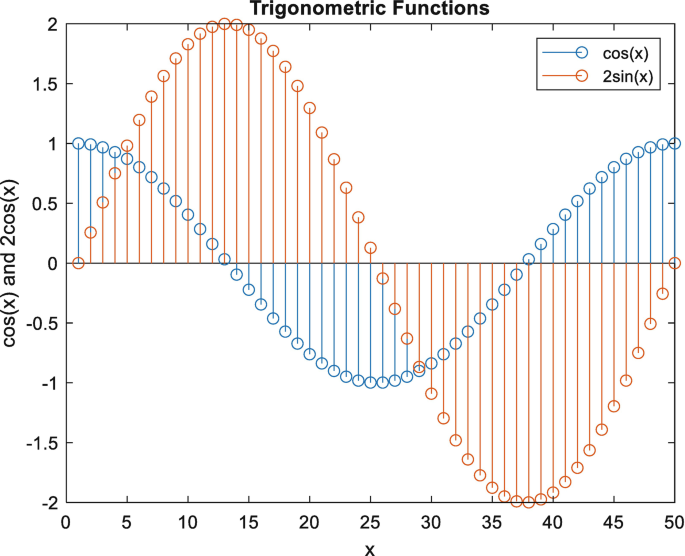

Physics

Functions describe motion, energy, and force.

Example:

Distance function:

[
d(t) = vt
]


Economics

Functions model cost, revenue, and profit.

Example:

[
Profit = Revenue – Cost
]


Computer Science

Functions appear in algorithms and programming.

Many programming languages implement functions as reusable code blocks.


Engineering

Functions model electrical signals, system responses, and mechanical systems.


Statistics

Probability distributions are functions.

Example:

Normal distribution.


Historical Development of Functions

The concept of function evolved over centuries.

Ancient mathematicians studied relationships between quantities without formal function notation.

In the 17th century, mathematicians like Leibniz introduced the term function.

Later mathematicians such as Euler formalized the concept.

Modern set theory defines functions using mappings between sets.


Importance of Functions in Mathematics

Functions are important because they:

  • Describe relationships between variables
  • Help model real-world systems
  • Provide tools for prediction and analysis
  • Serve as foundation for calculus and advanced mathematics

Nearly every branch of mathematics uses functions.


Conclusion

Functions are one of the most powerful and fundamental concepts in mathematics. They allow us to express relationships between quantities and analyze how one variable changes in response to another. Through algebraic expressions, graphs, tables, and mappings, functions provide multiple ways to understand and interpret mathematical relationships.
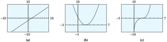
From simple linear equations to complex exponential and trigonometric models, functions form the backbone of mathematical analysis and scientific modeling. Their applications extend across numerous disciplines including physics, engineering, economics, computer science, and statistics.

Understanding functions enables mathematicians and scientists to explore patterns, solve problems, predict outcomes, and build mathematical models that explain the behavior of the world around us.

Mastery of functions provides the foundation for advanced mathematical topics such as calculus, differential equations, and mathematical modeling, making them an essential topic in the study of mathematics.


Tags