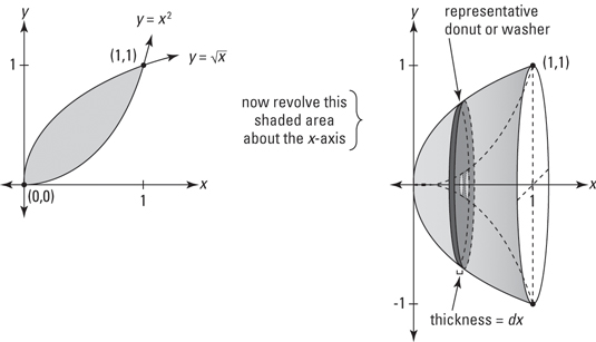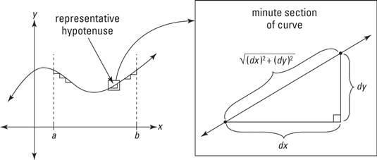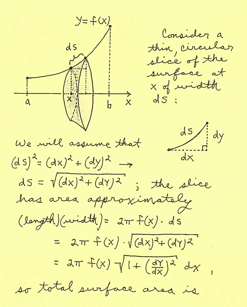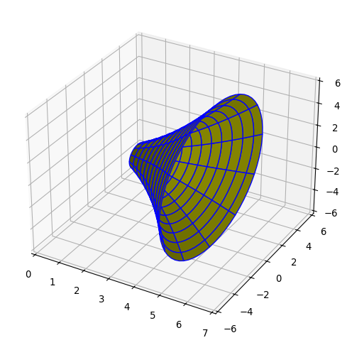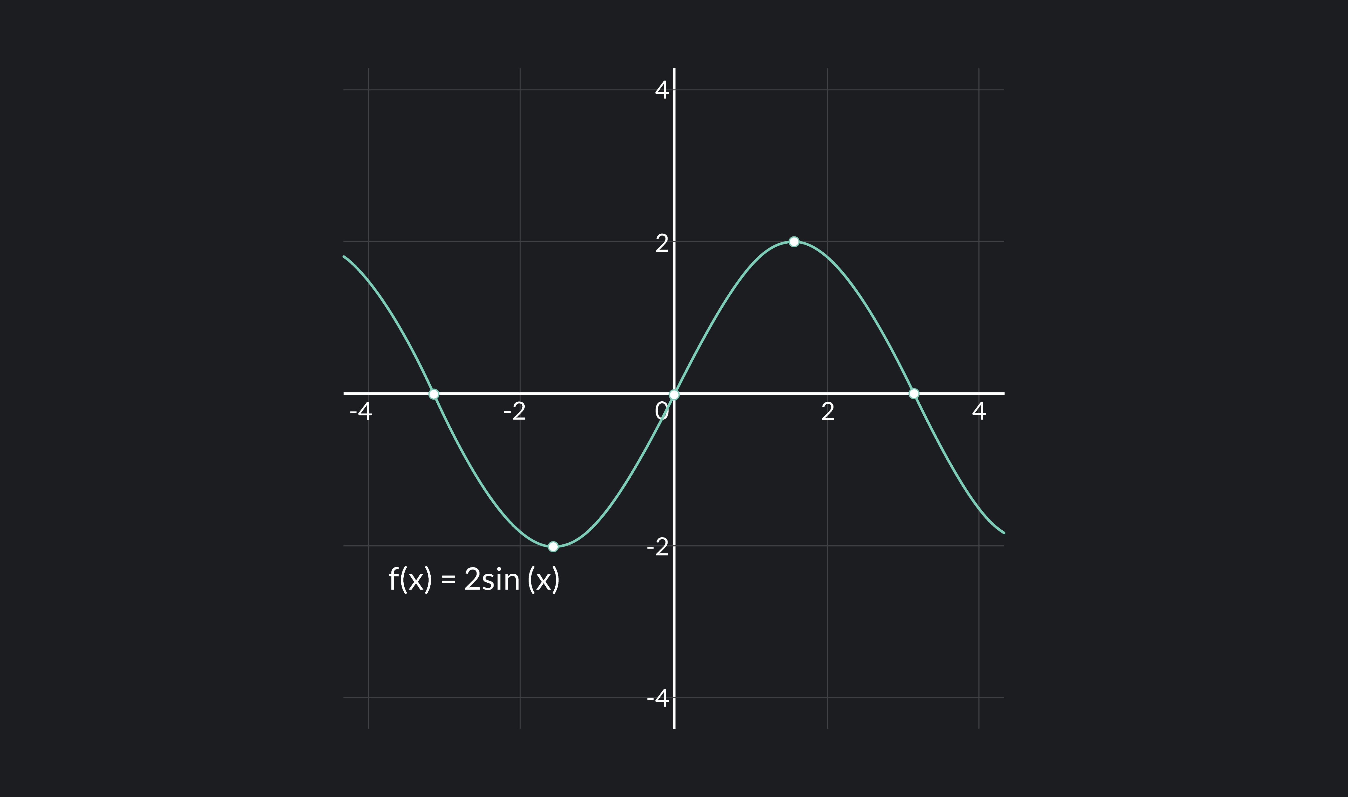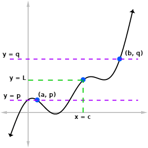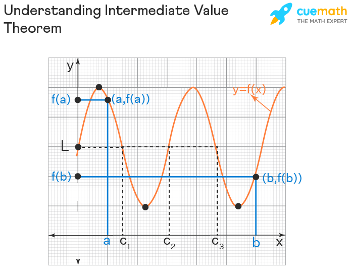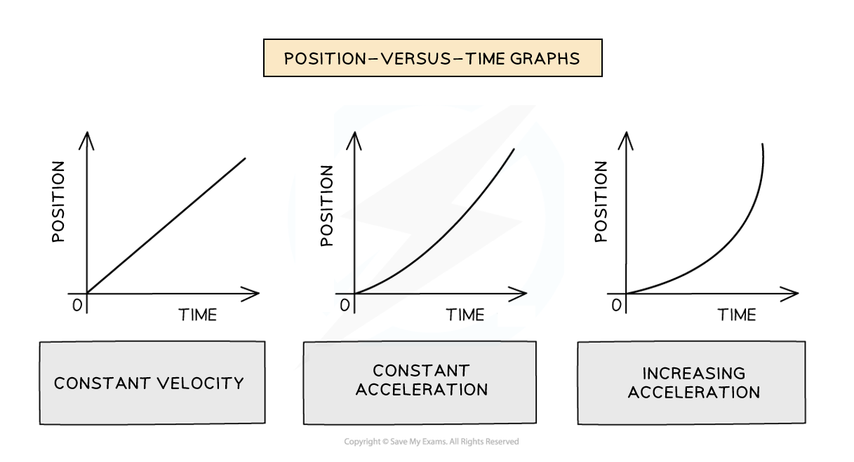
Category Archives: Mathematics

Applications of Integration in Mathematics

Image
Image
Image
Image

Introduction to Applications of Integration

Integration is one of the two fundamental operations in calculus, the other being differentiation. While differentiation measures the rate of change of a function, integration focuses on accumulation and total quantities. Integration is used to determine areas, volumes, lengths, and many other quantities that accumulate continuously.

The concept of integration originated from the problem of finding the area under a curve. Early mathematicians such as Isaac Newton and Gottfried Wilhelm Leibniz developed calculus to solve such problems. Integration provides a powerful mathematical tool for calculating quantities that cannot be easily measured using simple formulas.

Applications of integration appear in many fields including mathematics, physics, engineering, economics, biology, and statistics. For example, integration can be used to determine the distance traveled by an object when its velocity is known, calculate the work done by a variable force, determine the area between curves, and find the volume of complex shapes.

In mathematical notation, integration is represented by the symbol:

This symbol represents the summation of infinitely small quantities.

There are two main types of integration:

  1. Indefinite Integration
  2. Definite Integration

The definite integral has many important practical applications because it allows the calculation of exact numerical values for accumulated quantities.


Definite Integrals and Their Meaning

Image
Image
Image
Image

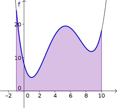
A definite integral represents the accumulation of quantities over a specific interval.

Mathematically, the definite integral of a function f(x) from a to b is written as:

∫ₐᵇ f(x) dx

This expression calculates the net area between the curve and the x-axis from x = a to x = b.

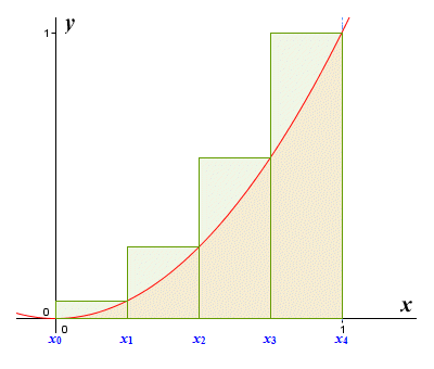
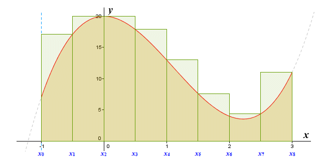
The concept behind definite integrals comes from Riemann sums, where the area under a curve is approximated using rectangles. As the number of rectangles increases and their width approaches zero, the approximation becomes exact.

This limit process leads to the definite integral.

Example:

If

f(x) = x²

Then the area under the curve from 0 to 2 is:

∫₀² x² dx

This evaluates to:

8/3

Thus, the area under the curve equals 8/3 square units.


Area Under a Curve

Image
Image
Image
Image

One of the most fundamental applications of integration is finding the area under a curve.

If a function f(x) is positive over the interval [a, b], the area under the curve is given by:

Area = ∫ₐᵇ f(x) dx

Example:

Find the area under the curve:

y = x

from x = 0 to x = 2.

Area:

∫₀² x dx

= [x²/2]₀²

= 2

Thus, the area is 2 square units.

Integration allows us to calculate areas even when the boundaries are curved rather than straight.


Area Between Two Curves

Image
Image
Image
Image

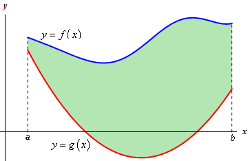
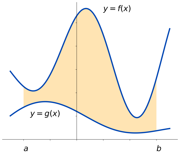
Integration can also determine the area between two curves.

If two functions are:

y = f(x)
y = g(x)

The area between them from x = a to x = b is:

Area = ∫ₐᵇ [f(x) − g(x)] dx

Example:

Find the area between:

y = x
y = x²

The curves intersect at x = 0 and x = 1.

Area:

∫₀¹ (x − x²) dx

= [x²/2 − x³/3]₀¹

= 1/2 − 1/3

= 1/6

Thus, the area between the curves is 1/6 square units.

This application is widely used in geometry and engineering.


Volume of Solids of Revolution
Image
Image
Image
Image

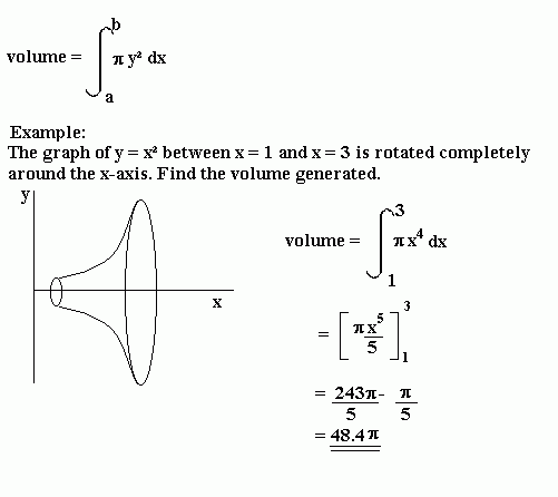
Integration is used to calculate the volume of three-dimensional solids.

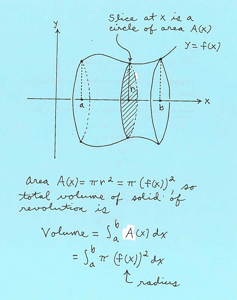
When a curve is rotated around an axis, it forms a solid of revolution.

Disk Method

Volume formula:

V = π ∫ₐᵇ [f(x)]² dx

Example:

Rotate y = x around the x-axis from 0 to 2.

Volume:

π ∫₀² x² dx

= π(8/3)

Washer Method

Used when there is a hollow region between curves.

These techniques help calculate volumes of complex shapes.


Length of a Curve
Image
Image
Image
Image

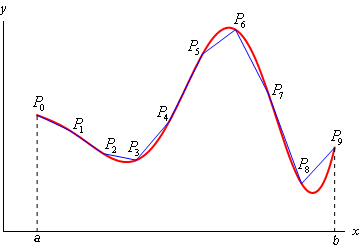
Integration can determine the length of curved lines.

The arc length formula for a function y = f(x) is:

L = ∫ₐᵇ √(1 + (dy/dx)²) dx

Example:

If

y = x²

Then:

dy/dx = 2x

Substitute into the formula to calculate the length.

Arc length calculations are important in engineering, physics, and computer graphics.


Surface Area of Solids
Image
Image
Image
Image

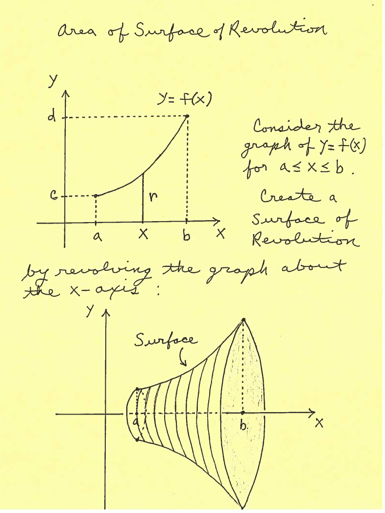
Integration is also used to find the surface area of solids of revolution.

Formula:

Surface Area = 2π ∫ₐᵇ f(x) √(1 + (f′(x))²) dx

This formula calculates the surface formed when a curve is rotated around an axis.

Such calculations are useful in designing containers, pipes, and mechanical components.


Work Done by a Variable Force
Image
Image
Image
Image

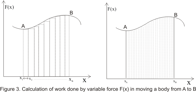
Integration is used in physics to calculate work done by variable forces.

Work is defined as:

W = ∫ F(x) dx

Example:

For a spring:

F = kx

Work required to stretch the spring:

W = ∫ kx dx

= (kx²)/2

Integration helps analyze mechanical systems and energy transfer.


Average Value of a Function
Image
Image
Image
Image

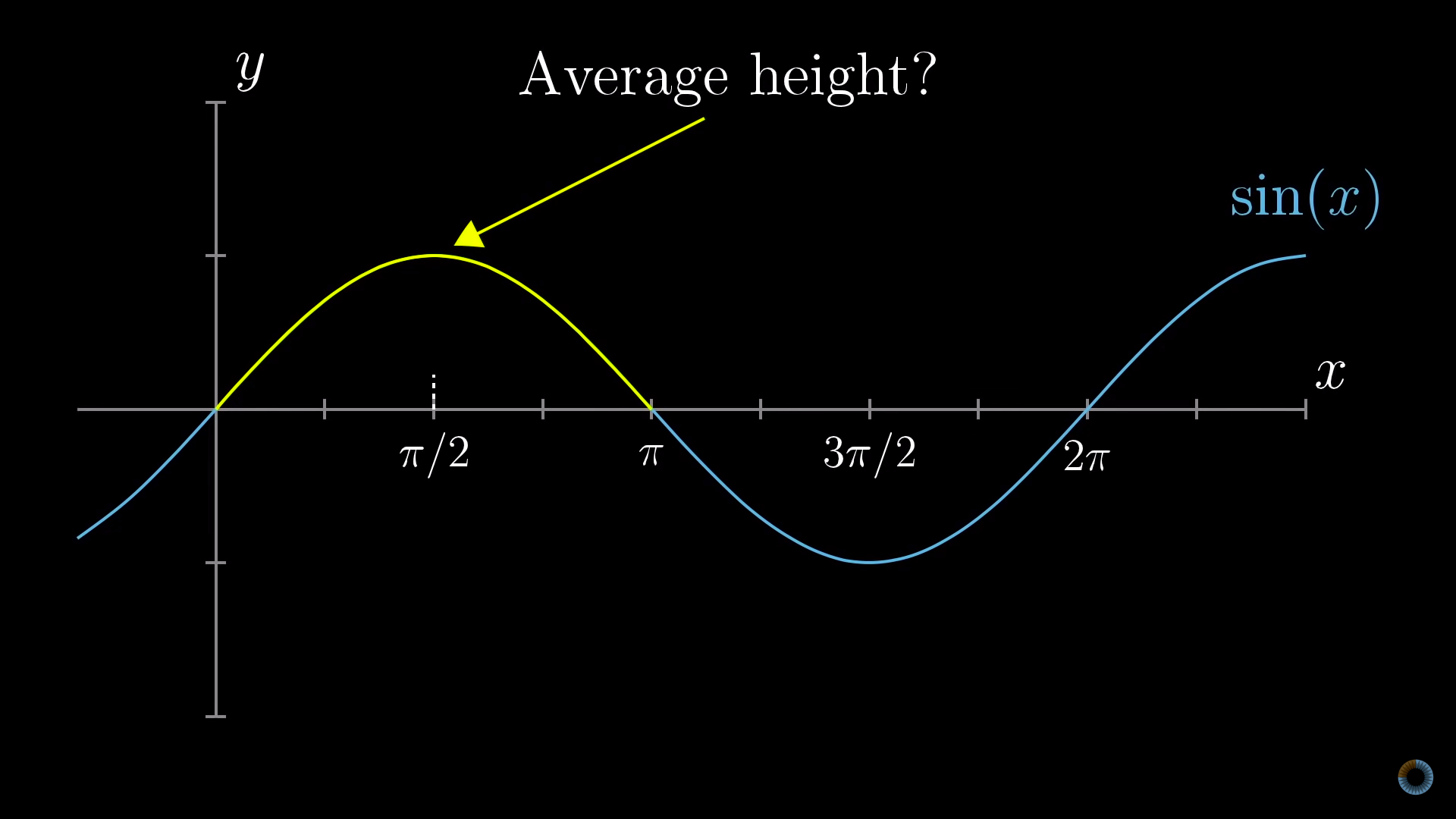
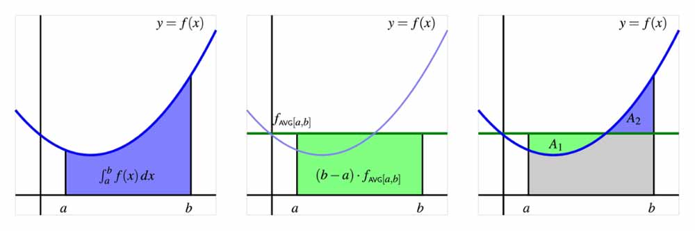
Integration can determine the average value of a function over an interval.

Formula:

Average value = (1/(b − a)) ∫ₐᵇ f(x) dx

Example:

For

f(x) = x²

on [0,2]:

Average value:

(1/2) ∫₀² x² dx

= 4/3

This concept is useful in statistics, physics, and economics.


Applications in Physics

Image
Image
Image
Image

Integration plays a major role in physics.

Examples include:

  • calculating displacement from velocity
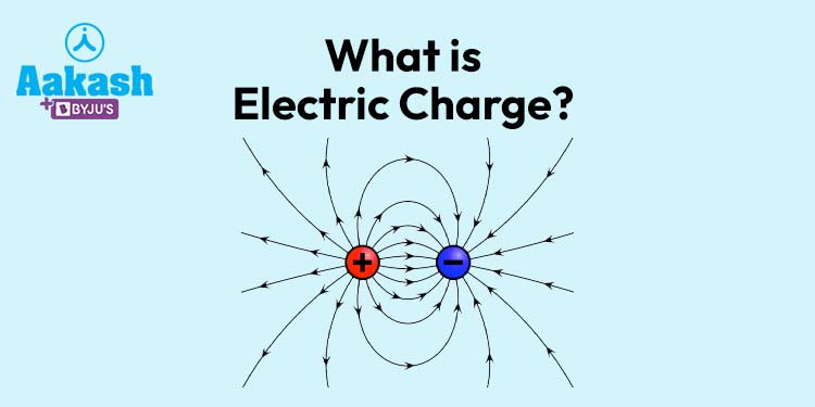
  • determining electric charge
  • finding fluid pressure
  • analyzing energy systems

For example:

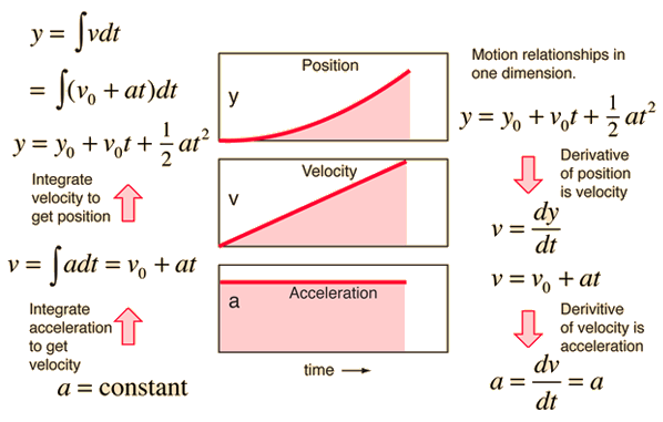
If velocity is known as a function of time:

v(t)

Then displacement is:

∫ v(t) dt


Applications in Economics

Image
Image
Image
Image

Integration is widely used in economics.

Examples include:

  • consumer surplus
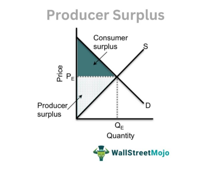
  • producer surplus
  • total revenue
  • accumulated cost

Consumer surplus is calculated as the area between the demand curve and market price.

These calculations help economists analyze market behavior.


Importance of Applications of Integration

Applications of integration demonstrate the power of calculus in solving real-world problems.

They allow mathematicians and scientists to calculate quantities that accumulate continuously, such as area, volume, work, and energy.

Integration provides essential tools for modeling physical systems, designing engineering structures, and analyzing economic data.

Because of its broad applicability, integration remains a key concept in mathematics and science.


Conclusion

Integration is a fundamental operation in calculus that focuses on accumulation and total quantities. The applications of integration include finding areas under curves, areas between curves, volumes of solids, arc lengths, surface areas, work done by variable forces, and many other quantities.

These applications play a crucial role in mathematics, physics, engineering, economics, and other scientific fields. Integration helps describe continuous processes and provides precise solutions to complex problems.

Understanding the applications of integration allows students and researchers to connect mathematical theory with real-world situations. Mastering these concepts provides a deeper understanding of calculus and its importance in modern science and technology.

Tags

Applications of Derivatives in Mathematics

Image
Image
Image
Image

Introduction to Applications of Derivatives

Derivatives are one of the most powerful tools in calculus. While the concept of differentiation focuses on determining the rate of change of a function, the applications of derivatives involve using derivatives to solve real-world problems in mathematics, physics, engineering, economics, biology, and many other disciplines.

In simple terms, derivatives help us understand how one quantity changes with respect to another. For example, derivatives can describe how fast a car is moving, how quickly a population is growing, or how profit changes with production levels. By analyzing derivatives, mathematicians and scientists can identify maximum and minimum values, determine slopes of curves, analyze motion, and optimize systems.

Applications of derivatives extend far beyond theoretical mathematics. They play a central role in modeling natural phenomena, designing engineering systems, optimizing business decisions, and analyzing scientific data.

The study of applications of derivatives helps students move from abstract mathematical theory to practical problem solving. It demonstrates how calculus can be used to understand real-world behavior and make informed decisions.


Rate of Change

Image
Image
Image
Image

One of the most fundamental applications of derivatives is measuring rate of change.

A derivative describes how rapidly one quantity changes with respect to another. For example:

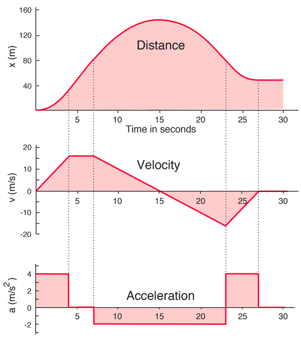
  • Velocity measures how position changes with time.
  • Acceleration measures how velocity changes with time.
  • Growth rate measures how a population changes over time.

Average Rate of Change

Average rate of change measures how a function changes over an interval.

Formula:

(f(b) − f(a)) / (b − a)

This represents the slope of the line connecting two points on the curve.

Instantaneous Rate of Change

Instantaneous rate of change describes how the function changes at a specific moment.

This is given by the derivative:

dy/dx

For example, if the position of a moving object is given by:

s(t) = t²

The velocity is:

v(t) = ds/dt = 2t

This means the velocity increases linearly with time.


Tangent and Normal to Curves

Image
Image
Image
Image

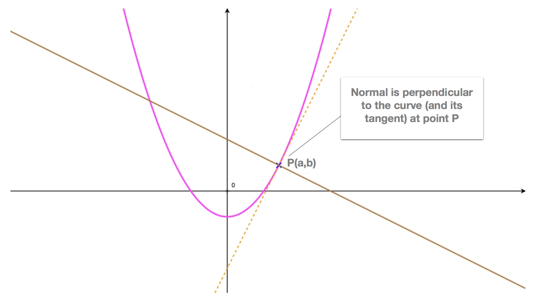
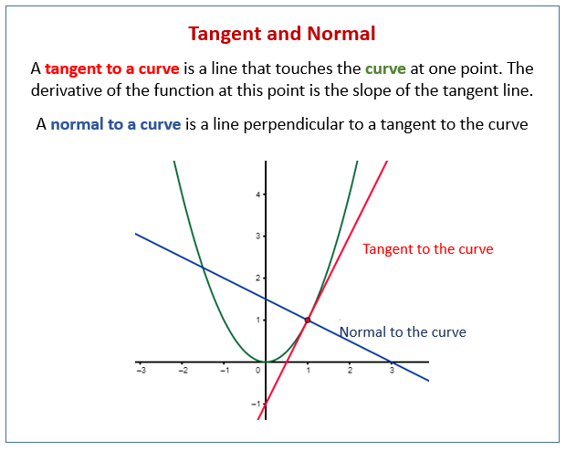
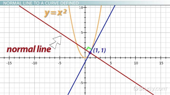
Derivatives are used to determine the equations of tangent and normal lines to curves.

Tangent Line

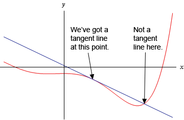
A tangent line touches a curve at exactly one point and has the same slope as the curve at that point.

If:

y = f(x)

Then the slope of the tangent is:

dy/dx

The equation of the tangent line at point (a, f(a)) is:

y − f(a) = f′(a)(x − a)

Normal Line

The normal line is perpendicular to the tangent line.

If the slope of the tangent is m, the slope of the normal is:

−1/m

These concepts are useful in geometry, physics, and engineering.


Increasing and Decreasing Functions

Image
Image
Image
Image

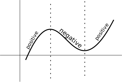
Derivatives help determine whether a function is increasing or decreasing.

If:

f′(x) > 0

The function is increasing.

If:

f′(x) < 0

The function is decreasing.

This information helps analyze the behavior of graphs and predict trends.

For example, if the derivative of a profit function is positive, profit is increasing as production increases.


Maxima and Minima (Optimization)

Image
Image
Image
Image

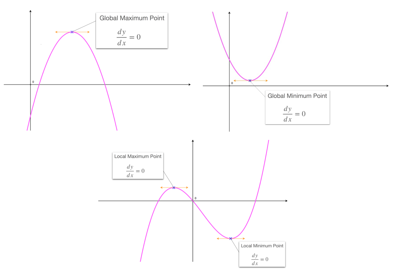
One of the most important applications of derivatives is finding maximum and minimum values.

These values are also known as extrema.

Critical Points

Critical points occur where:

f′(x) = 0

or

f′(x) is undefined.

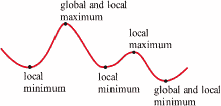
These points may correspond to maxima, minima, or saddle points.

First Derivative Test

If the derivative changes from positive to negative, the point is a maximum.

If the derivative changes from negative to positive, the point is a minimum.

Example

Consider the function:

f(x) = −x² + 4x

Derivative:

f′(x) = −2x + 4

Set derivative to zero:

−2x + 4 = 0

x = 2

Thus, the function has a maximum at x = 2.

Optimization problems are widely used in engineering, economics, and business.


Concavity and Points of Inflection

Image
Image
Image
Image

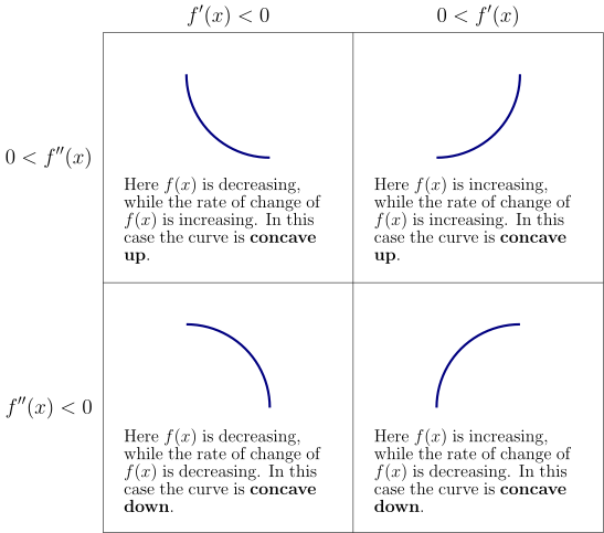
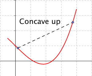
The second derivative helps determine the concavity of a function.

If:

f″(x) > 0

The graph is concave upward.

If:

f″(x) < 0

The graph is concave downward.

Points of Inflection

A point of inflection occurs where the concavity changes.

This happens when:

f″(x) = 0

These points help understand the shape of curves.


Curve Sketching

Image
Image
Image
Image

Derivatives play a major role in curve sketching.

To sketch a curve, we analyze:

  • intercepts
  • asymptotes
  • increasing/decreasing intervals
  • maxima and minima
  • concavity
  • inflection points

Using derivatives, mathematicians can determine the overall shape of a graph without plotting many points.

This technique is widely used in calculus and mathematical modeling.


Motion in Physics

Image
Image
Image
Image

Derivatives are essential for describing motion in physics.

If:

s(t) = position

Then:

v(t) = ds/dt = velocity

a(t) = dv/dt = acceleration

These relationships allow physicists to study motion of objects such as cars, rockets, and planets.

Example:

If

s(t) = t³

Velocity:

v(t) = 3t²

Acceleration:

a(t) = 6t


Optimization in Economics

Image
Image
Image
Image

In economics, derivatives help determine optimal production levels.

Marginal Cost

Marginal cost is the derivative of the cost function.

Marginal Revenue

Marginal revenue is the derivative of the revenue function.

Profit Maximization

Profit is maximized when:

Marginal revenue = marginal cost.

These calculations help businesses determine efficient production levels.


Applications in Engineering

Image
Image
Image
Image

Engineers use derivatives in many areas.

Examples include:

  • designing machines
  • analyzing electrical signals
  • studying heat transfer
  • optimizing structures

Derivatives help engineers model systems and improve efficiency.


Applications in Biology and Medicine

Image
Image
Image
Image

Derivatives are used to analyze biological processes.

Examples include:

  • population growth
  • spread of diseases
  • rate of chemical reactions
  • drug concentration in the body

Mathematical models based on derivatives help scientists understand biological systems.


Importance of Applications of Derivatives

Applications of derivatives demonstrate how calculus can solve real-world problems.

They help:

  • analyze motion
  • optimize systems
  • study natural phenomena
  • improve engineering designs
  • model economic behavior

Understanding these applications makes calculus more practical and meaningful.


Conclusion

Derivatives are powerful mathematical tools used to analyze rates of change, slopes of curves, and optimal values in various problems. The applications of derivatives extend across many fields including physics, engineering, economics, biology, and computer science.

Through derivatives, mathematicians can determine tangent lines, analyze increasing and decreasing behavior of functions, find maximum and minimum values, study concavity, and model real-world phenomena.

Because of their versatility and wide range of applications, derivatives remain one of the most important concepts in calculus and applied mathematics.

Mastering the applications of derivatives enables students to solve complex problems, understand dynamic systems, and apply mathematical reasoning to real-world situations.


Tags

Differentiation in Mathematics (Calculus)

Image
Image
Image
Image

Introduction to Differentiation

Differentiation is one of the central concepts in calculus and mathematical analysis. It is used to study how a function changes with respect to its input. In simple terms, differentiation measures the rate at which a quantity changes. The result of differentiation is called the derivative of a function.

Differentiation allows mathematicians and scientists to determine slopes of curves, rates of change, and optimal values in various problems. It has numerous applications in physics, engineering, economics, biology, computer science, and many other fields.

For example, when a car moves along a road, its position changes over time. Differentiation can be used to determine the velocity of the car by measuring how quickly its position changes. Similarly, differentiation can determine acceleration, growth rates, and trends in data.

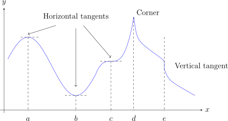
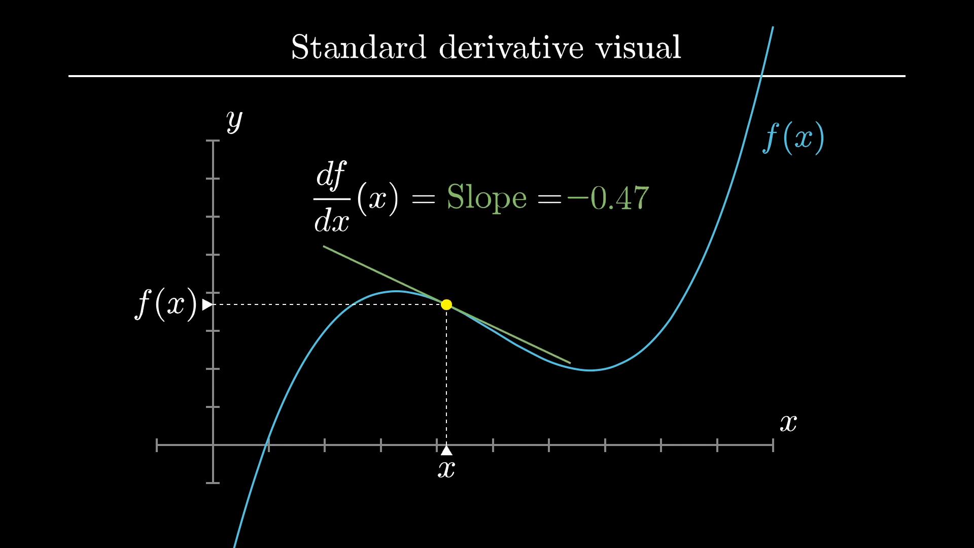
The derivative of a function represents the slope of the tangent line to the curve at a given point. It provides information about how steep the curve is and whether the function is increasing or decreasing at that point.

Mathematically, if a function is represented by f(x), its derivative is often written as:

f′(x) or dy/dx

This derivative describes how the value of the function changes as x changes.

Differentiation forms the basis of many advanced topics in calculus such as optimization, curve sketching, differential equations, and mathematical modeling.


Concept of Rate of Change

Image
Image
Image
Image

The idea of differentiation comes from the concept of rate of change.

Rate of change describes how one quantity varies with respect to another. For example:

  • Speed describes how distance changes with time.
  • Population growth describes how population changes over time.
  • Temperature variation describes how temperature changes during the day.

There are two types of rate of change.

Average Rate of Change

The average rate of change measures how a function changes over an interval.

Average rate of change formula:

(f(b) − f(a)) / (b − a)

This represents the slope of the line connecting two points on the curve.

Instantaneous Rate of Change

The instantaneous rate of change measures how the function changes at a specific point.

This is found using derivatives and represents the slope of the tangent line.

Differentiation focuses on the instantaneous rate of change.


Definition of Derivative

Image
Image
Image
Image

The derivative of a function is defined using limits.

Mathematically:

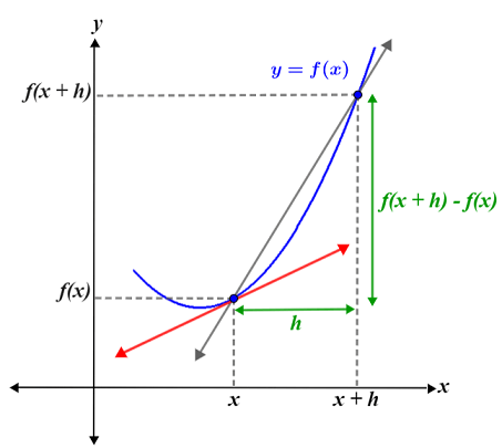
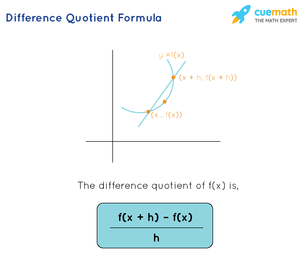
f′(x) = lim (h → 0) [f(x + h) − f(x)] / h

This expression is called the difference quotient.

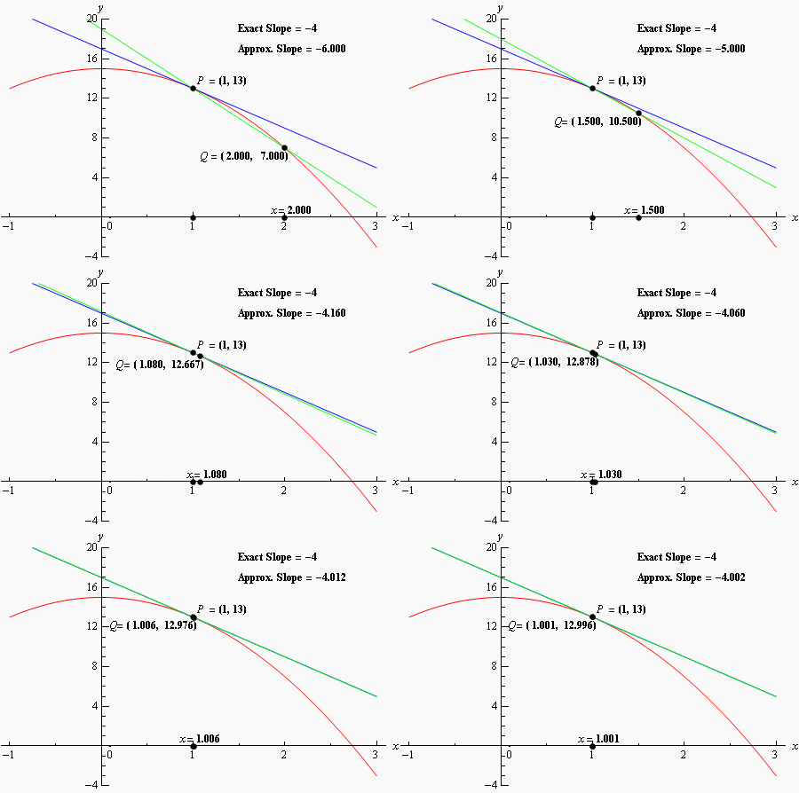
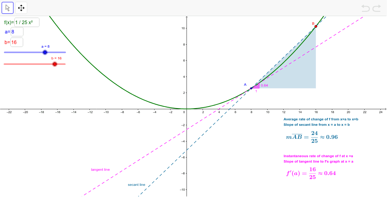
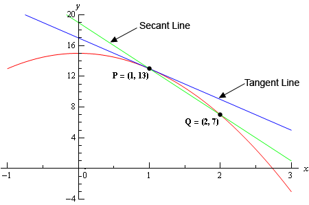
It measures the slope of the secant line between two points on the curve. As the distance between the points approaches zero, the secant line becomes the tangent line.

Thus, the derivative represents the slope of the tangent line at a specific point.

Example:

Let:

f(x) = x²

Then:

f′(x) = 2x

This means the slope of the curve at any point x is 2x.


Geometric Interpretation of Differentiation

Image
Image
Image
Image

Geometrically, differentiation represents the slope of the tangent line to a curve at a given point.

A tangent line touches the curve at exactly one point and represents the direction of the curve at that point.

If the slope is positive, the function is increasing.

If the slope is negative, the function is decreasing.

If the slope is zero, the function may have a maximum or minimum point.

This interpretation helps in understanding the shape and behavior of graphs.


Basic Rules of Differentiation

Image
Image
Image
Image

Several rules simplify the process of differentiation.

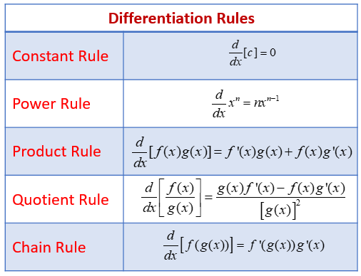
Constant Rule

The derivative of a constant is zero.

d/dx (c) = 0

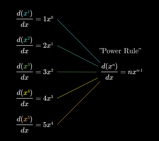
Power Rule

d/dx (xⁿ) = nxⁿ⁻¹

Example:

d/dx (x³) = 3x²

Sum Rule

d/dx (f + g) = f′ + g′

Difference Rule

d/dx (f − g) = f′ − g′

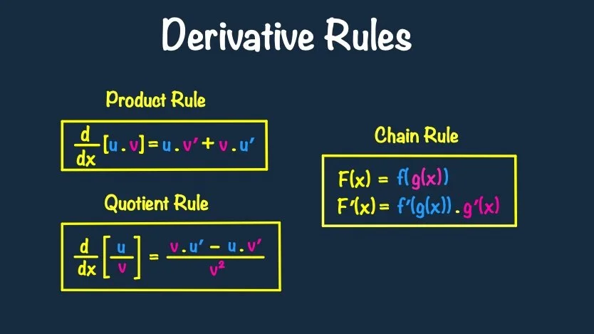
Product Rule

d/dx (fg) = f′g + fg′

Quotient Rule

d/dx (f/g) = (f′g − fg′)/g²

These rules help differentiate complex expressions efficiently.


Chain Rule

Image
Image
Image
Image

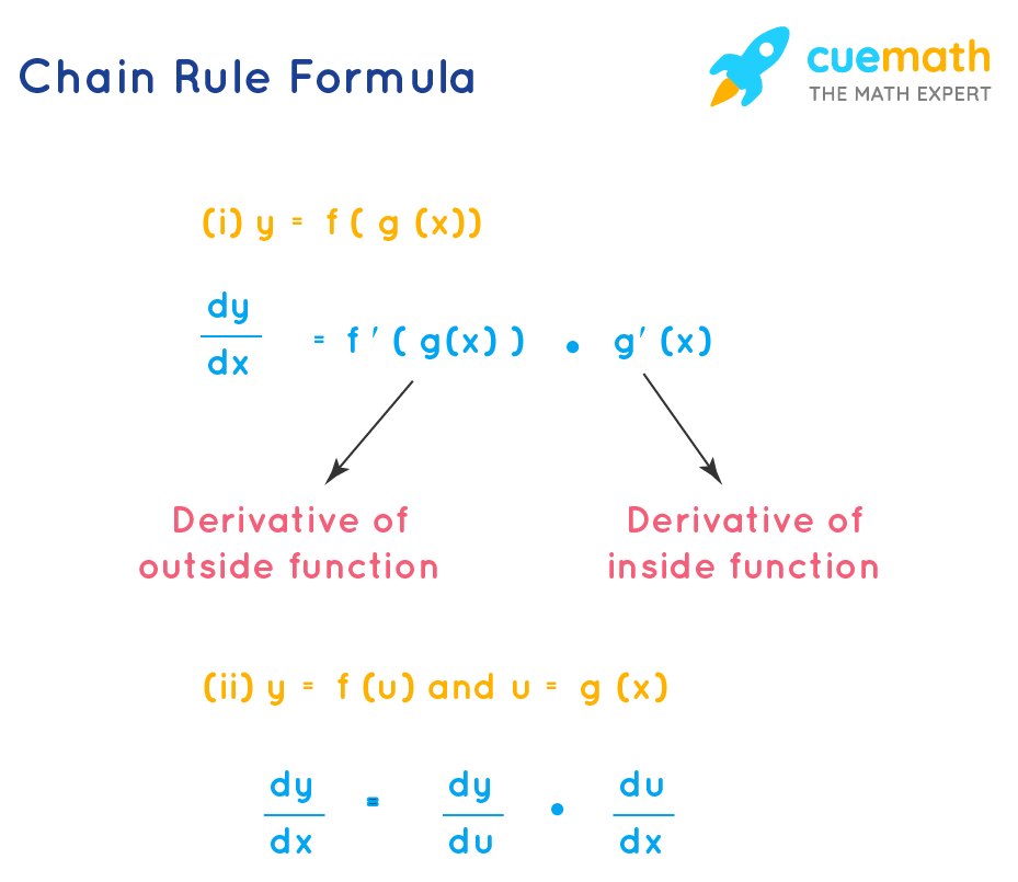
The chain rule is used to differentiate composite functions.

If:

y = f(g(x))

Then:

dy/dx = f′(g(x)) × g′(x)

Example:

If

y = (x² + 1)³

Then:

dy/dx = 3(x² + 1)² × 2x

Chain rule is essential for differentiating functions involving nested expressions.


Derivatives of Common Functions

Image
Image
Image
Image

Important derivatives include:

Derivative of sine:

d/dx (sin x) = cos x

Derivative of cosine:

d/dx (cos x) = −sin x

Derivative of tangent:

d/dx (tan x) = sec²x

Derivative of exponential:

d/dx (eˣ) = eˣ

Derivative of logarithm:

d/dx (ln x) = 1/x

These derivatives are widely used in calculus.


Higher-Order Derivatives

Image
Image
Image
Image

The derivative of a derivative is called a higher-order derivative.

Second derivative:

f″(x)

Third derivative:

f‴(x)

The second derivative describes acceleration or concavity of the graph.

If f″(x) > 0, the curve is concave upward.

If f″(x) < 0, the curve is concave downward.

Higher-order derivatives are important in physics and engineering.


Applications of Differentiation

Image
Image
Image
Image

Differentiation has many practical applications.

Physics

Used to calculate velocity and acceleration.

Engineering

Used to design machines and analyze systems.

Economics

Used to determine marginal cost and profit.

Biology

Used to study population growth rates.

Computer Science

Used in machine learning algorithms and optimization.


Maxima and Minima

Image
Image
Image
Image

Differentiation helps determine maximum and minimum values of functions.

Steps:

  1. Find derivative.
  2. Set derivative equal to zero.
  3. Solve for critical points.

These points represent maxima, minima, or saddle points.

Optimization problems rely heavily on derivatives.


Importance of Differentiation

Differentiation is essential for understanding change and motion in mathematics and science.

It helps analyze curves, optimize systems, and model real-world phenomena. Without differentiation, modern physics, engineering, and economics would not be possible.

Differentiation also forms the basis for differential equations, which describe many natural processes.


Conclusion

Differentiation is a fundamental concept in calculus that measures the rate of change of a function. It provides a powerful mathematical tool for analyzing curves, determining slopes, and solving optimization problems.

The derivative represents the slope of the tangent line and describes how a function changes at a particular point. Differentiation is closely connected to limits and continuity and plays a crucial role in many areas of mathematics and science.

Understanding differentiation allows students and researchers to model real-world processes, analyze data, and solve complex problems involving change. Because of its wide range of applications, differentiation remains one of the most important tools in mathematics and applied sciences.


Tags

Continuity in Mathematics (Calculus)

Image
Image
Image
Image

Introduction to Continuity

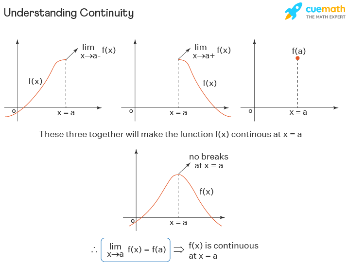
Continuity is one of the most important concepts in calculus and mathematical analysis. It describes how a function behaves without sudden breaks, jumps, or gaps. In simple terms, a function is continuous if its graph can be drawn without lifting the pencil from the paper.

The concept of continuity is closely related to limits and is fundamental for understanding many advanced topics in calculus such as derivatives, integrals, and differential equations. Continuity ensures that small changes in the input of a function produce small changes in the output, which makes mathematical models predictable and stable.

In real-world situations, many physical phenomena are continuous. For example, temperature changes gradually over time, the position of a moving object changes smoothly, and the flow of water in a river does not suddenly jump from one location to another. Mathematics uses the concept of continuity to represent these smooth transitions.

Understanding continuity helps mathematicians analyze functions, identify points of discontinuity, and determine whether a function behaves smoothly over a given interval.


Intuitive Understanding of Continuity

Image
Image
Image
Image

The intuitive idea of continuity is simple: a function is continuous if its graph has no interruptions.

Imagine drawing a curve on a sheet of paper. If you can draw the entire graph without lifting your pen, the function is continuous. If you must lift the pen because the graph has a break or gap, then the function is discontinuous at that point.

There are several situations where discontinuities occur:

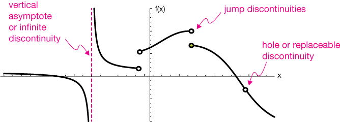
  • A hole in the graph
  • A jump between two values
  • An infinite break

These interruptions prevent the function from being continuous at certain points.

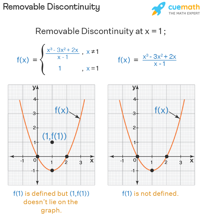
For example, consider the function:

f(x) = (x² − 1)/(x − 1)

If we substitute x = 1 directly, the expression becomes undefined. However, if we simplify the expression:

(x² − 1)/(x − 1) = x + 1

The simplified function behaves normally except at x = 1, where there is a hole in the graph. This type of discontinuity is called a removable discontinuity.


Formal Definition of Continuity

Image
Image
Image
Image

In calculus, continuity is defined using limits.

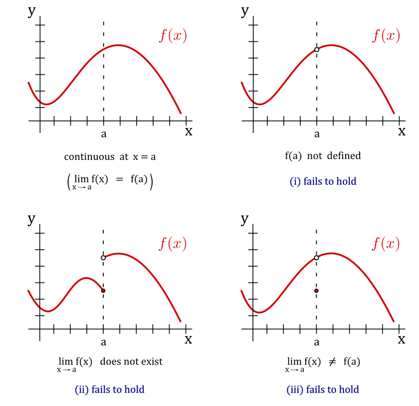
A function f(x) is continuous at a point x = a if the following three conditions are satisfied:

  1. The function f(a) is defined.
  2. The limit of the function as x approaches a exists.
  3. The limit of the function equals the value of the function.

Mathematically:

lim (x → a) f(x) = f(a)

If these conditions hold true, the function is continuous at the point x = a.

If any of these conditions fail, the function is discontinuous at that point.

This definition ensures that the function behaves smoothly at the point under consideration.


Types of Discontinuities

Image
Image
Image
Image

A function may fail to be continuous in several ways. These are called discontinuities.

Removable Discontinuity

A removable discontinuity occurs when the function has a hole in the graph but can be made continuous by redefining the function at that point.

Example:

f(x) = (x² − 1)/(x − 1)

The function has a hole at x = 1, which can be removed by defining f(1) = 2.

Jump Discontinuity

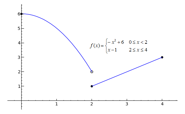
A jump discontinuity occurs when the left-hand limit and right-hand limit are different.

Example:

lim (x → a⁻) f(x) ≠ lim (x → a⁺) f(x)

This results in a sudden jump in the graph.

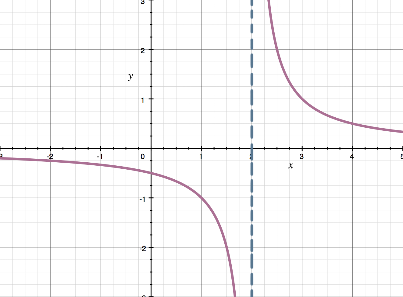
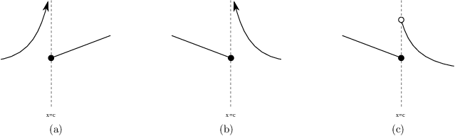
Infinite Discontinuity

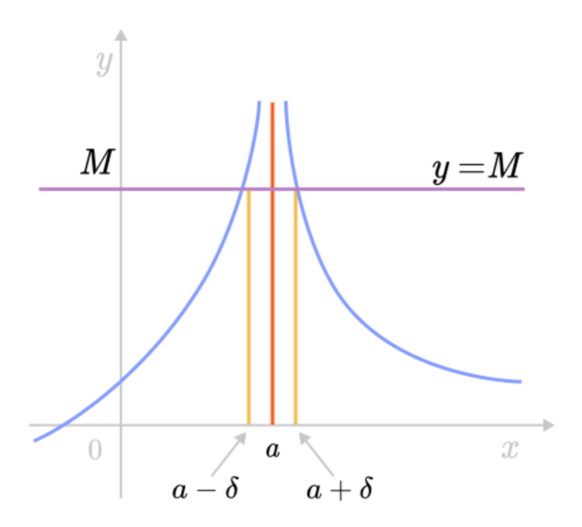
An infinite discontinuity occurs when the function approaches infinity near a certain point.

Example:

f(x) = 1/x

At x = 0, the function approaches infinity.

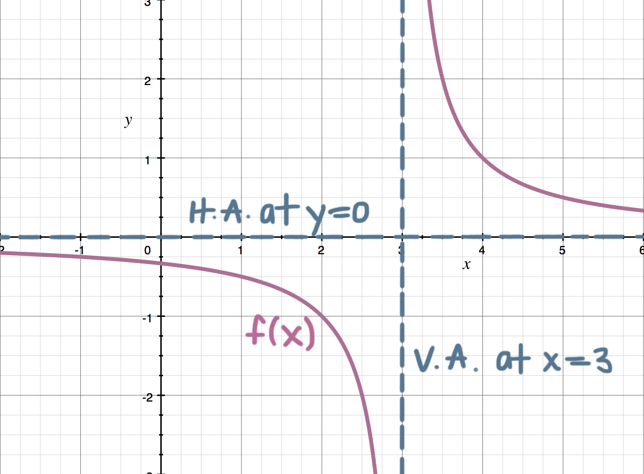
This creates a vertical asymptote in the graph.


Continuity on an Interval

Image
Image
Image

A function is continuous on an interval if it is continuous at every point within that interval.

Continuity on an Open Interval

A function is continuous on (a, b) if it is continuous at every point between a and b.

Continuity on a Closed Interval

A function is continuous on [a, b] if:

  • It is continuous on (a, b)
  • The right-hand limit exists at a
  • The left-hand limit exists at b

Many functions such as polynomials and trigonometric functions are continuous over their entire domains.


Continuous Functions

Image
Image
Image
Image

Several types of functions are naturally continuous.

Polynomial Functions

All polynomial functions are continuous for all real numbers.

Example:

f(x) = x³ + 2x + 1

Rational Functions

Rational functions are continuous wherever the denominator is not zero.

Trigonometric Functions

Functions such as sine and cosine are continuous everywhere.

Exponential Functions

Exponential functions are continuous across their entire domain.

Logarithmic Functions

Logarithmic functions are continuous for positive values of x.

Understanding which functions are continuous helps simplify many mathematical problems.


Properties of Continuous Functions

Continuous functions have several important properties.

Sum of Continuous Functions

If two functions are continuous, their sum is also continuous.

Product of Continuous Functions

The product of two continuous functions is continuous.

Quotient of Continuous Functions

The quotient of two continuous functions is continuous provided the denominator is not zero.

Composition of Continuous Functions

If f(x) and g(x) are continuous, then f(g(x)) is also continuous.

These properties help mathematicians analyze complex functions.


Intermediate Value Theorem

Image
Image
Image
Image

One of the most important results related to continuity is the Intermediate Value Theorem (IVT).

The theorem states:

If a function is continuous on a closed interval [a, b] and takes values f(a) and f(b), then the function must take every value between f(a) and f(b).

In simple terms, a continuous function cannot skip values.

Example:

If a continuous function has values:

f(1) = 2
f(4) = 10

Then the function must take every value between 2 and 10 somewhere between x = 1 and x = 4.

This theorem is widely used to prove the existence of solutions to equations.


Applications of Continuity

Image
Image
Image
Image

Continuity has many practical applications in science and engineering.

Physics

Continuity helps describe motion, velocity, and acceleration of objects.

Engineering

Engineers use continuous functions to model systems and signals.

Economics

Continuous models help describe economic growth and market trends.

Computer Science

Continuity is used in optimization algorithms and machine learning models.

Environmental Science

Continuous functions help model temperature changes and climate behavior.


Importance of Continuity in Calculus

Continuity plays a crucial role in calculus because many operations depend on it.

For example:

  • Derivatives require continuity.
  • Integrals depend on continuous functions.
  • Many mathematical theorems assume continuity.

A function that is not continuous may behave unpredictably, making mathematical analysis difficult.

Thus, continuity provides a foundation for analyzing smooth and predictable behavior in functions.


Continuity and Differentiability

Image
Image
Image
Image

Differentiability and continuity are closely related.

If a function is differentiable at a point, it must also be continuous at that point.

However, the reverse is not always true.

A function may be continuous but not differentiable.

Example:

f(x) = |x|

The graph of this function is continuous at x = 0 but has a sharp corner, so it is not differentiable there.

This relationship highlights the importance of continuity in calculus.


Conclusion

Continuity is a fundamental concept in mathematics that describes functions that change smoothly without breaks, gaps, or jumps. It is closely related to limits and forms the basis for many topics in calculus, including derivatives and integrals.

A function is continuous at a point if the limit of the function exists and equals the value of the function at that point. When continuity fails, discontinuities such as holes, jumps, or infinite breaks may occur.

Understanding continuity helps mathematicians and scientists analyze functions, model real-world phenomena, and solve complex mathematical problems. Because many natural processes change smoothly over time, continuity plays a vital role in physics, engineering, economics, and other scientific fields.

Mastering the concept of continuity provides a strong foundation for advanced mathematical studies and helps students develop deeper insights into the behavior of functions.


Tags

Limits in Mathematics (Calculus)

Image
Image
Image
Image

Introduction to Limits

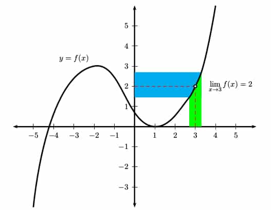
Limits are one of the most fundamental concepts in calculus and mathematical analysis. They describe the behavior of a function as its input approaches a particular value. Instead of focusing on the exact value of a function at a specific point, limits examine what value the function is approaching.

The concept of limits forms the foundation for many advanced mathematical ideas, including derivatives, integrals, continuity, and infinite series. Without limits, the development of calculus would not be possible.

In simple terms, a limit answers the question:

What value does a function approach as the input gets closer and closer to a certain number?

For example, consider a function f(x). If the values of f(x) become closer to a number L as x approaches a value a, then we say that the limit of f(x) as x approaches a equals L.

This is written mathematically as:

lim (x → a) f(x) = L

This expression means that the function f(x) approaches the value L as x approaches the number a.

Limits allow mathematicians to analyze behavior near a point even if the function is not defined exactly at that point. This makes limits a powerful tool for studying functions and their properties.


Intuitive Understanding of Limits

Image
Image
Image
Image

To understand limits intuitively, imagine a function represented by a curve on a graph. As the x-values get closer and closer to a particular point, the y-values may approach a specific number.

For example, consider the function:

f(x) = (x² − 1)/(x − 1)

If we substitute x = 1 directly into the function, we get:

0/0

This expression is undefined. However, if we simplify the function:

(x² − 1)/(x − 1) = (x − 1)(x + 1)/(x − 1)

Canceling (x − 1):

f(x) = x + 1

Now, if x approaches 1:

f(x) approaches 2.

Therefore:

lim (x → 1) (x² − 1)/(x − 1) = 2

Even though the function is not defined at x = 1, the limit exists and equals 2.

This demonstrates how limits describe the behavior of functions near a point.


Formal Definition of a Limit

Image
Image
Image
Image

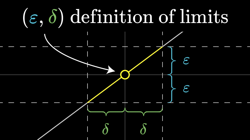
The rigorous mathematical definition of limits was developed using the epsilon-delta definition.

The definition states:

The limit of f(x) as x approaches a equals L if for every small positive number ε (epsilon), there exists another small positive number δ (delta) such that whenever the distance between x and a is less than δ, the distance between f(x) and L is less than ε.

Mathematically:

If 0 < |x − a| < δ then |f(x) − L| < ε

This definition ensures that the function values can be made arbitrarily close to L by choosing x sufficiently close to a.

Although the epsilon-delta definition may appear complex, it provides a precise way to define limits mathematically.


One-Sided Limits

Image
Image
Image
Image

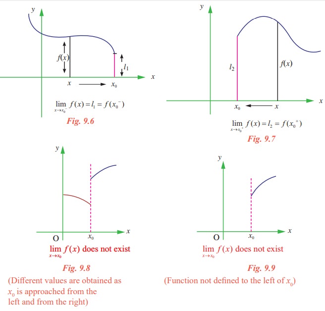
Sometimes it is necessary to study limits from only one side of a point.

These are called one-sided limits.

Left-Hand Limit

The left-hand limit occurs when x approaches a from values less than a.

Notation:

lim (x → a⁻) f(x)

Right-Hand Limit

The right-hand limit occurs when x approaches a from values greater than a.

Notation:

lim (x → a⁺) f(x)

For a limit to exist, the left-hand and right-hand limits must be equal.

Example:

If

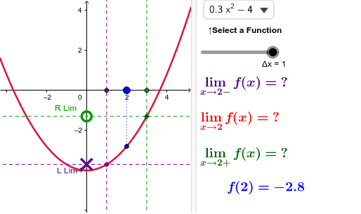
lim (x → 2⁻) f(x) = 3
lim (x → 2⁺) f(x) = 3

Then

lim (x → 2) f(x) = 3

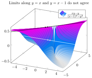
If the two one-sided limits are different, the limit does not exist.


Limits at Infinity

Image
Image
Image
Image

Limits can also describe the behavior of functions as x becomes extremely large or extremely small.

These are called limits at infinity.

Example:

lim (x → ∞) (1/x) = 0

As x becomes larger and larger, the value of 1/x becomes smaller and approaches zero.

Another example:

lim (x → ∞) (2x + 1)/(x + 3) = 2

To determine such limits, we divide numerator and denominator by x.

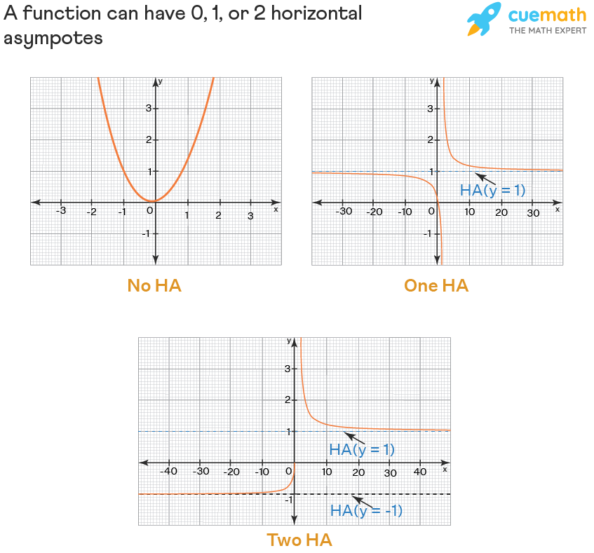
Limits at infinity help identify horizontal asymptotes in graphs.


Algebra of Limits

Image
Image
Image
Image

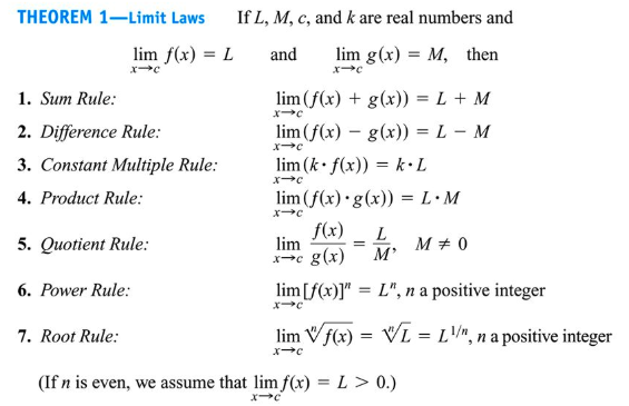
Several rules make it easier to evaluate limits.

Let:

lim f(x) = L
lim g(x) = M

Then:

Sum Rule

lim [f(x) + g(x)] = L + M

Difference Rule

lim [f(x) − g(x)] = L − M

Product Rule

lim [f(x)g(x)] = LM

Quotient Rule

lim [f(x)/g(x)] = L/M

provided M ≠ 0.

Constant Rule

lim c = c

These rules simplify the evaluation of complex limits.


Techniques for Evaluating Limits

Image
Image
Image
Image

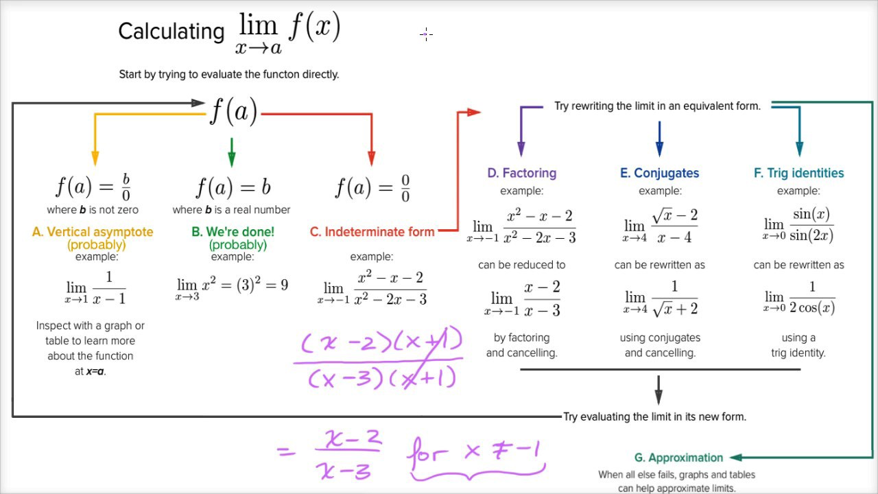
Different techniques are used to evaluate limits.

Substitution

Direct substitution works if the function is continuous at the point.

Factorization

Factorizing expressions can eliminate undefined forms.

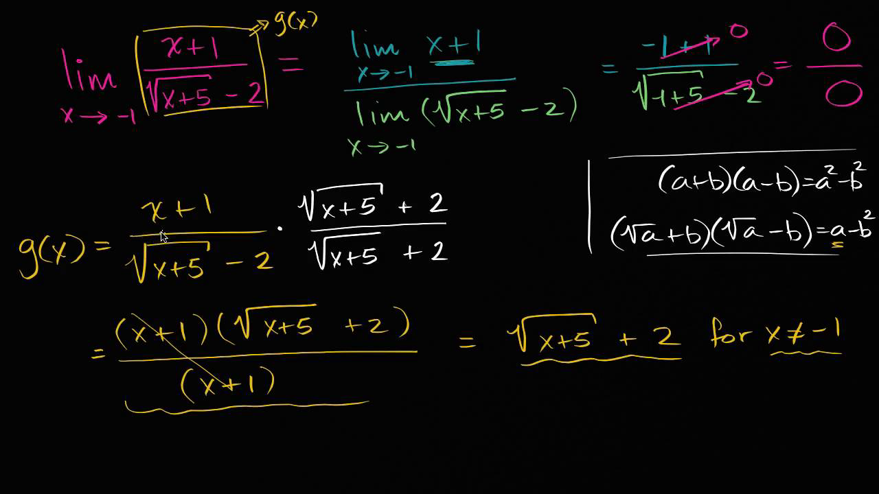
Rationalization

Multiplying by conjugates can simplify radical expressions.

Common Denominator

Combining fractions helps simplify expressions.

Trigonometric Limits

Some limits use special trigonometric formulas.

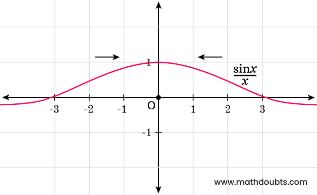
Example:

lim (x → 0) sin x / x = 1

These techniques help solve many calculus problems.


Important Standard Limits

Image
Image
Image
Image

Several limits are fundamental in calculus.

Important examples include:

lim (x → 0) sin x / x = 1

lim (x → 0) (1 − cos x)/x = 0

lim (x → ∞) (1 + 1/x)^x = e

These limits are frequently used in calculus and mathematical analysis.


Limits and Continuity

Image
Image
Image
Image

Limits are closely related to the concept of continuity.

A function is continuous at a point if:

  1. The function is defined at that point.
  2. The limit exists at that point.
  3. The limit equals the function value.

Mathematically:

lim (x → a) f(x) = f(a)

If these conditions are satisfied, the function is continuous at x = a.

Continuity is essential for calculus operations such as differentiation and integration.


Applications of Limits

Image
Image
Image
Image

Limits have many practical applications.

Calculating Derivatives

The derivative of a function is defined using limits.

Physics

Limits help describe motion, velocity, and acceleration.

Engineering

Engineers use limits in modeling systems and signals.

Economics

Limits are used in marginal analysis and optimization.

Computer Science

Limits help analyze algorithms and computational complexity.


Importance of Limits in Calculus

Limits form the foundation of calculus.

They are used to define:

  • derivatives
  • integrals
  • continuity
  • infinite series

Without limits, the mathematical study of change and accumulation would not be possible.

Limits allow mathematicians to analyze behavior at very small scales and understand instantaneous rates of change.


Conclusion

Limits are a fundamental concept in mathematics that describe how functions behave as their input approaches a specific value. They provide the foundation for calculus and play a crucial role in defining derivatives, integrals, and continuity.

Understanding limits helps mathematicians and scientists analyze functions, model real-world phenomena, and solve complex problems involving change and motion. Limits are widely used in physics, engineering, economics, and computer science.

Mastering limits is an essential step for students studying calculus and advanced mathematics, as it opens the door to deeper mathematical understanding and powerful analytical tools.


Tags

Heights and Distances in Trigonometry

Image
Image
Image
Image

Introduction to Heights and Distances

Heights and distances is an important topic in trigonometry that deals with determining the height of objects and the distance between objects using trigonometric ratios. This concept is widely applied in fields such as surveying, navigation, engineering, architecture, astronomy, and physics. It allows us to measure quantities that cannot be measured directly by using mathematical relationships involving angles and triangles.

In everyday life, we often need to determine the height of tall objects such as buildings, towers, mountains, trees, and bridges. Similarly, we may need to calculate distances across rivers, valleys, or other obstacles where direct measurement is not possible. Trigonometry provides powerful tools to solve such problems using angles of elevation, angles of depression, and trigonometric ratios.

The fundamental idea behind heights and distances is the formation of a right triangle between the observer, the object being observed, and the horizontal ground. By measuring certain angles and distances, trigonometric ratios such as sine, cosine, and tangent can be used to determine unknown values.

Understanding heights and distances is essential for solving many practical problems in mathematics and science. It combines geometric reasoning with trigonometric formulas to provide accurate measurements in real-world situations.


Basic Concepts Used in Heights and Distances

Image
Image
Image
Image

Before studying heights and distances, it is necessary to understand some basic trigonometric concepts.

Right Triangle

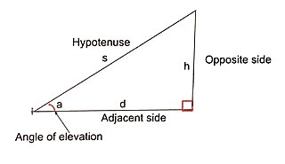
A right triangle is a triangle that contains one angle equal to 90°. The sides of a right triangle are called:

  • Hypotenuse
  • Opposite side
  • Adjacent side

Hypotenuse

The hypotenuse is the longest side of the triangle and lies opposite the right angle.

Opposite Side

The opposite side is the side opposite the angle under consideration.

Adjacent Side

The adjacent side is the side next to the angle but not the hypotenuse.

Trigonometric Ratios

Three important trigonometric ratios are used in heights and distances problems.

Sine

sin θ = opposite / hypotenuse

Cosine

cos θ = adjacent / hypotenuse

Tangent

tan θ = opposite / adjacent

Among these ratios, tangent is the most commonly used in heights and distances problems because it directly relates height and horizontal distance.


Angle of Elevation

Image
Image
Image
Image

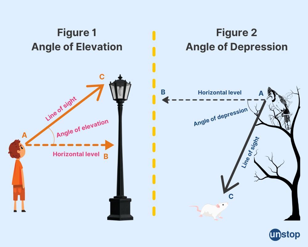
The angle of elevation is the angle between the horizontal line and the line of sight when an observer looks upward at an object.

When a person standing on the ground looks up at the top of a building, tower, or mountain, the angle formed between the horizontal line and the line of sight is called the angle of elevation.

Example of Angle of Elevation

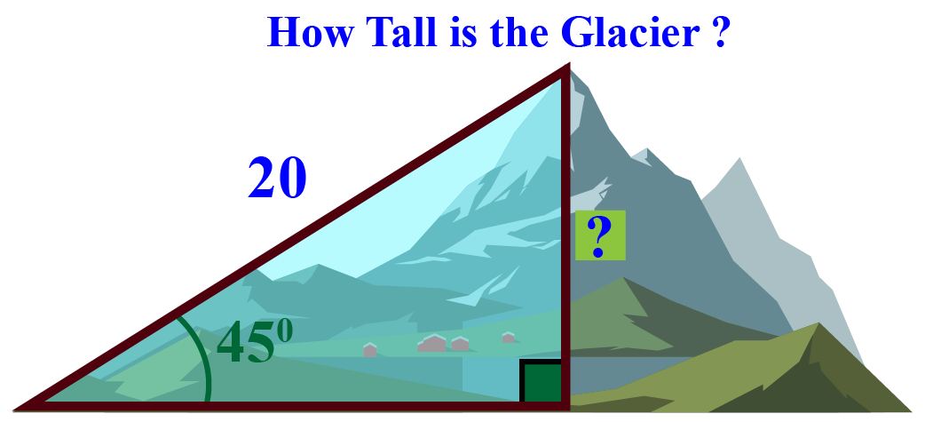
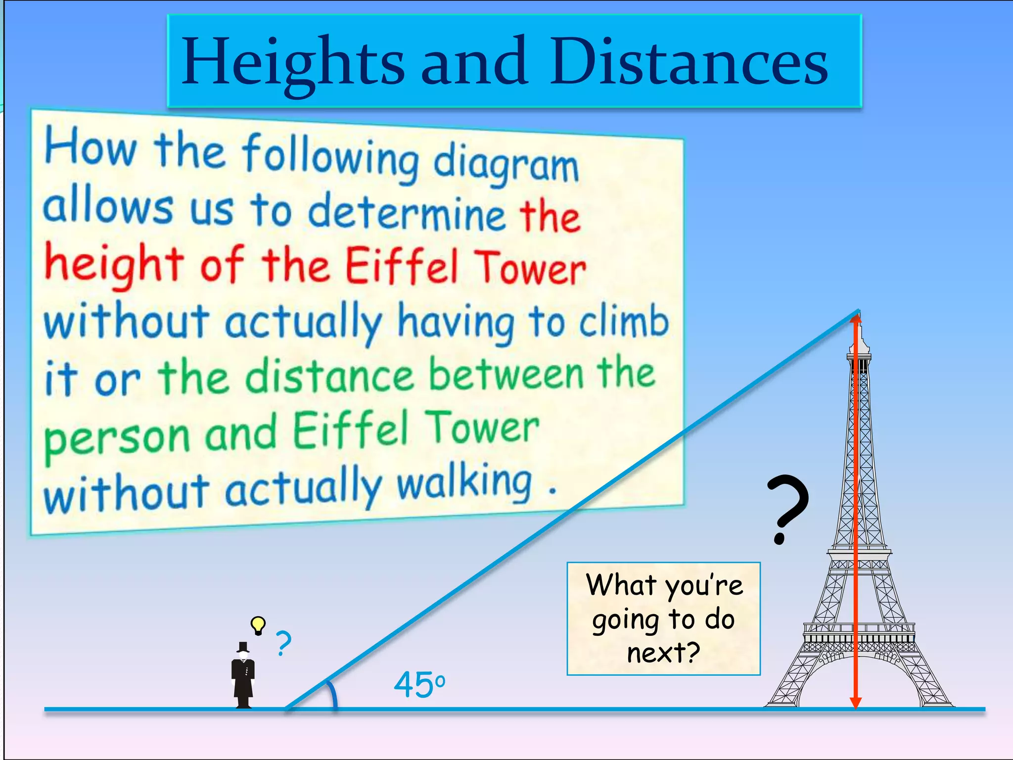
Suppose a person stands 20 meters away from a tower and observes the top of the tower at an angle of elevation of 45°.

Using trigonometry:

tan θ = height / distance

tan 45° = height / 20

Since tan 45° = 1

height = 20 meters

Thus, the height of the tower is 20 meters.

Real-Life Situations

Angle of elevation is used in situations such as:

  • Measuring the height of buildings
  • Determining the height of trees
  • Calculating the height of mountains
  • Surveying land

It allows measurements to be taken without physically climbing or measuring the object.


Angle of Depression

Image
Image
Image
Image

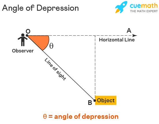
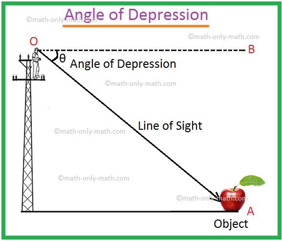
The angle of depression is the angle between the horizontal line and the line of sight when an observer looks downward at an object.

For example, if a person standing on top of a building looks down at a car on the ground, the angle between the horizontal line and the line of sight is called the angle of depression.

An important concept is that the angle of depression is equal to the angle of elevation because they are alternate interior angles formed by parallel lines.

Example of Angle of Depression

Suppose a lighthouse is 40 meters high. The angle of depression of a boat from the top of the lighthouse is 30°.

Using trigonometry:

tan 30° = height / distance

1/√3 = 40 / distance

distance = 40√3 meters

Thus, the boat is approximately 69.28 meters away from the lighthouse.


Horizontal Distance

Image
Image
Image
Image

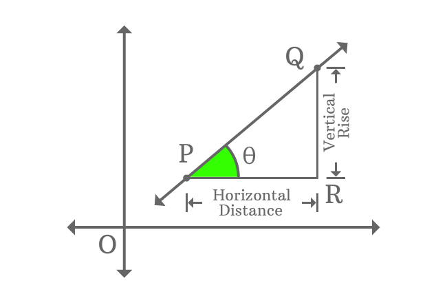
Horizontal distance refers to the distance between the observer and the base of the object along the ground.

This distance is usually measured directly using measuring tools or estimated using surveying techniques.

Once the horizontal distance and the angle of elevation are known, the height of the object can be calculated using trigonometric ratios.

Example

Distance from tower = 30 meters
Angle of elevation = 60°

Using tangent:

tan 60° = height / 30

√3 = height / 30

height = 30√3

height ≈ 51.96 meters

Thus, the height of the tower is approximately 52 meters.


Applications of Heights and Distances

Image
Image
Image
Image

Heights and distances have numerous practical applications.

Surveying

Surveyors use trigonometry to measure land areas and elevations. Instruments such as the theodolite help measure angles accurately.

Architecture

Architects use trigonometric calculations to determine building heights and slopes.

Navigation

Pilots and sailors use trigonometry to determine positions and distances.

Astronomy

Astronomers measure distances between celestial objects using trigonometric methods.

Engineering

Engineers use these calculations when designing bridges, towers, and other structures.


Solving Heights and Distances Problems

Many problems involve forming a right triangle and applying trigonometric ratios.

Step-by-Step Method

  1. Draw a diagram representing the situation.
  2. Identify the angle of elevation or depression.
  3. Label the sides of the triangle.
  4. Choose the appropriate trigonometric ratio.
  5. Substitute values and solve.

Example Problem

A tree stands on level ground. A person stands 15 meters away from the base of the tree. The angle of elevation of the top of the tree is 30°.

Find the height of the tree.

Using tangent:

tan 30° = height / 15

1/√3 = height / 15

height = 15 / √3

height ≈ 8.66 meters

Thus, the height of the tree is approximately 8.66 meters.


Multiple Observation Problems

Image
Image
Image
Image

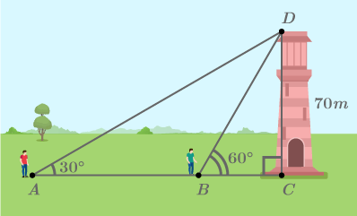
Sometimes heights are determined using two observation points.

Example

A tower is observed from two points on the same line with the base of the tower. The angles of elevation are 30° and 60°.

Let:

Distance from first point = x
Distance from second point = x + d

Using tangent formulas, equations can be formed to determine the height of the tower.

This method is commonly used in surveying and engineering measurements.


Real-Life Examples of Heights and Distances

Heights and distances problems appear in many everyday situations.

Measuring Building Height

Surveyors measure building heights without climbing them by using angles of elevation.

Determining Mountain Height

Mountains are measured using trigonometric calculations based on observation angles.

Aircraft Navigation

Pilots use trigonometry to determine altitude and distance.

Bridge Construction

Engineers calculate angles and distances to design stable structures.

Satellite Communication

Satellite positioning uses trigonometric calculations to determine distance from Earth.


Importance of Heights and Distances in Mathematics

Heights and distances play a significant role in mathematics education because they demonstrate how theoretical concepts can solve real-world problems.

This topic helps students develop:

  • spatial reasoning
  • problem-solving skills
  • understanding of trigonometric relationships

It also serves as a bridge between pure mathematics and applied mathematics.

Students learn how mathematical models can represent real-life situations and provide accurate solutions.


Advantages of Using Trigonometry for Measurements

Trigonometry provides several advantages for measuring heights and distances.

  1. Allows measurement of inaccessible objects
  2. Provides high accuracy
  3. Requires minimal equipment
  4. Can be applied to large-scale measurements

Because of these advantages, trigonometry remains an essential tool in science and engineering.


Conclusion

Heights and distances is an important application of trigonometry that allows us to calculate heights and distances of objects that cannot be measured directly. By using angles of elevation, angles of depression, and trigonometric ratios, unknown values can be determined accurately.

The concepts involved include right triangles, trigonometric ratios, horizontal distances, and angle measurements. These ideas are applied in surveying, architecture, navigation, engineering, and astronomy.

Understanding heights and distances helps students see the practical use of mathematics in everyday life. It demonstrates how trigonometry provides solutions to real-world measurement problems and highlights the power of mathematical reasoning.


Tags

Inverse Trigonometric Functions

Image
Image
Image
Image

Introduction to Inverse Trigonometric Functions

Inverse trigonometric functions are mathematical functions that reverse the operations of the basic trigonometric functions. While trigonometric functions such as sine, cosine, and tangent take an angle as input and produce a ratio as output, inverse trigonometric functions perform the opposite process: they take a ratio as input and return the corresponding angle.

For example, consider the equation:

sin θ = 0.5

The inverse sine function helps determine the value of θ that satisfies this equation. In this case:

θ = sin⁻¹(0.5)

Thus, inverse trigonometric functions are used to determine angles when the trigonometric ratio is known.

Inverse trigonometric functions are commonly written using the notation:

  • sin⁻¹(x) or arcsin(x)
  • cos⁻¹(x) or arccos(x)
  • tan⁻¹(x) or arctan(x)

It is important to note that sin⁻¹(x) does not mean 1/sin(x). Instead, it represents the inverse function of sine.

Inverse trigonometric functions play an essential role in mathematics, physics, engineering, computer science, navigation, and many scientific disciplines. They are especially important in calculus, trigonometric equations, coordinate geometry, and analytic geometry.


Basic Concept of Inverse Functions

Image
Image
Image
Image

Before understanding inverse trigonometric functions, it is necessary to understand the concept of inverse functions.

A function f(x) and its inverse f⁻¹(x) reverse each other’s operations.

If:

y = f(x)

Then:

x = f⁻¹(y)

For example:

If:

y = sin x

Then:

x = sin⁻¹ y

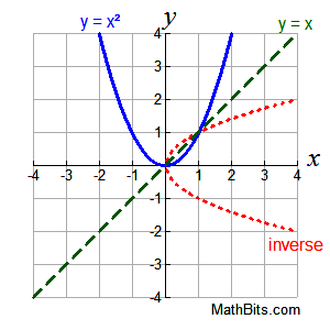
Graphically, the graph of a function and its inverse are reflections of each other across the line:

y = x

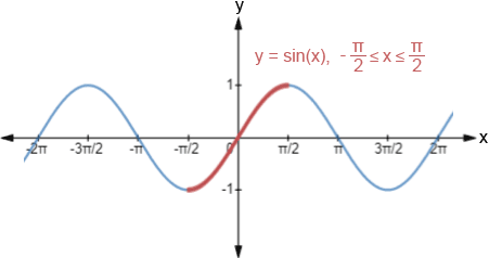
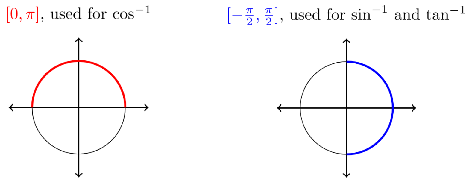
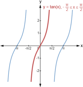
However, trigonometric functions are periodic and not one-to-one across their entire domain. Therefore, to define inverse trigonometric functions, we restrict the domain of trigonometric functions so that each output corresponds to exactly one input.

This restricted interval ensures that inverse trigonometric functions behave like proper functions.


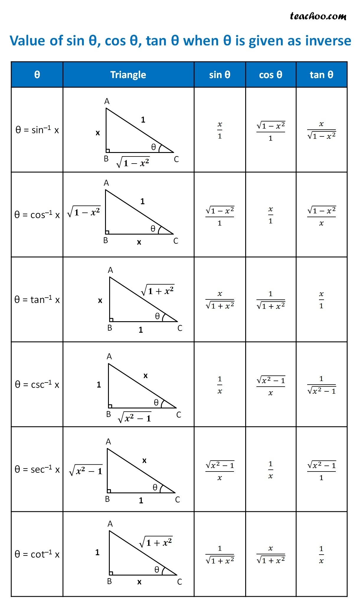
Types of Inverse Trigonometric Functions

Image
Image
Image
Image

There are six inverse trigonometric functions corresponding to the six trigonometric functions:

  1. arcsin(x) or sin⁻¹(x)
  2. arccos(x) or cos⁻¹(x)
  3. arctan(x) or tan⁻¹(x)
  4. arccot(x) or cot⁻¹(x)
  5. arcsec(x) or sec⁻¹(x)
  6. arccsc(x) or csc⁻¹(x)

Each inverse function returns the angle whose trigonometric ratio equals the given number.

These functions are essential in solving trigonometric equations and modeling real-world phenomena involving angles.


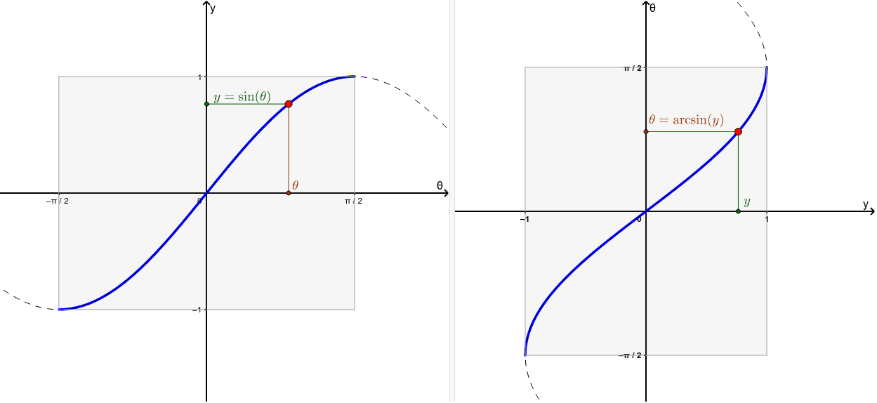
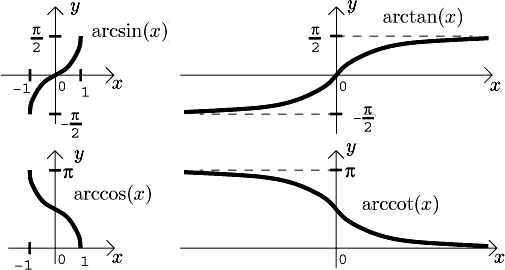
Inverse Sine Function (arcsin)

Image
Image
Image
Image

The inverse sine function determines the angle whose sine value is given.

Definition:

θ = sin⁻¹(x)

means

sin θ = x

Domain and Range

Domain:
-1 ≤ x ≤ 1

Range:
−π/2 ≤ θ ≤ π/2

or

−90° ≤ θ ≤ 90°

Example

sin⁻¹(1/2)

The angle whose sine is 1/2 is:

30°

Thus:

sin⁻¹(1/2) = 30°

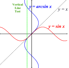
Graph Characteristics

The arcsin graph:

  • passes through (0,0)
  • increases continuously
  • ranges from −π/2 to π/2

The arcsin function is widely used in geometry and calculus.


Inverse Cosine Function (arccos)

Image
Image
Image
Image

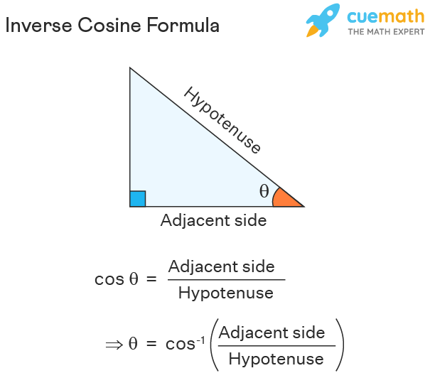
The inverse cosine function finds the angle whose cosine value equals a given number.

Definition:

θ = cos⁻¹(x)

means:

cos θ = x

Domain

-1 ≤ x ≤ 1

Range

0 ≤ θ ≤ π

or

0° ≤ θ ≤ 180°

Example

cos⁻¹(1/2)

The angle whose cosine equals 1/2 is:

60°

Thus:

cos⁻¹(1/2) = 60°

The arccos function is decreasing and is often used in geometry and vector calculations.


Inverse Tangent Function (arctan)

Image
Image
Image
Image

The inverse tangent function determines the angle whose tangent equals a given number.

Definition:

θ = tan⁻¹(x)

means:

tan θ = x

Domain

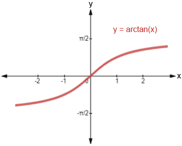
All real numbers

Range

−π/2 < θ < π/2

Example

tan⁻¹(1)

Since:

tan 45° = 1

Therefore:

tan⁻¹(1) = 45°

The arctan function is widely used in physics and engineering to calculate angles from slopes.


Other Inverse Trigonometric Functions

Image
Image
Image
Image

Besides arcsin, arccos, and arctan, there are three additional inverse trigonometric functions.

Inverse Cotangent

θ = cot⁻¹(x)

Range:

0 < θ < π

Inverse Secant

θ = sec⁻¹(x)

Domain:

|x| ≥ 1

Inverse Cosecant

θ = csc⁻¹(x)

Domain:

|x| ≥ 1

These functions are less frequently used but still important in advanced mathematics and calculus.


Properties of Inverse Trigonometric Functions

Inverse trigonometric functions satisfy several important properties.

Composition Property

sin(sin⁻¹ x) = x

cos(cos⁻¹ x) = x

tan(tan⁻¹ x) = x

Example

sin(sin⁻¹(0.6)) = 0.6

Angle Relationships

sin⁻¹ x + cos⁻¹ x = π/2

tan⁻¹ x + cot⁻¹ x = π/2

These identities are useful for simplifying expressions.


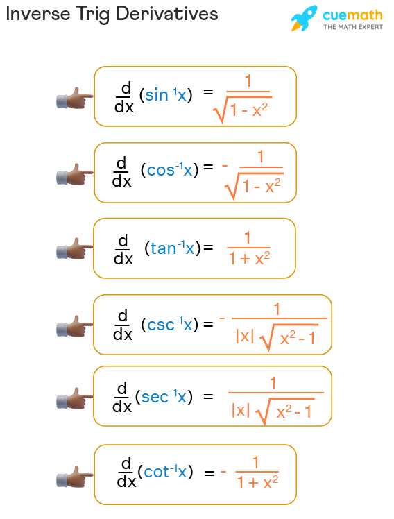
Derivatives of Inverse Trigonometric Functions

Inverse trigonometric functions play a major role in calculus.

Important derivatives include:

d/dx (sin⁻¹ x) = 1 / √(1 − x²)

d/dx (cos⁻¹ x) = −1 / √(1 − x²)

d/dx (tan⁻¹ x) = 1 / (1 + x²)

These formulas are essential in integration and differential calculus.


Applications of Inverse Trigonometric Functions

Inverse trigonometric functions are widely used in many scientific and engineering fields.

Geometry

They help determine unknown angles when side lengths are known.

Physics

They are used in:

  • projectile motion
  • wave analysis
  • optics

Engineering

Engineers use inverse trigonometric functions in:

  • robotics
  • structural design
  • signal processing

Navigation

They help determine direction and location in GPS systems.

Computer Graphics

Inverse trigonometric functions are used to compute rotations and angles in 3D modeling.


Importance in Mathematics

Inverse trigonometric functions are essential in advanced mathematics topics such as:

  • calculus
  • differential equations
  • complex analysis
  • Fourier analysis

They allow mathematicians to solve equations involving trigonometric ratios and analyze periodic behavior.


Conclusion

Inverse trigonometric functions are mathematical functions that determine angles from trigonometric ratios. They reverse the operations of sine, cosine, tangent, and other trigonometric functions.

The most commonly used inverse trigonometric functions are arcsin, arccos, and arctan. These functions have specific domains and ranges to ensure they remain one-to-one functions.

Inverse trigonometric functions are essential tools in solving trigonometric equations, studying calculus, analyzing wave motion, and modeling geometric relationships. Their applications extend across many scientific and engineering disciplines.

A strong understanding of inverse trigonometric functions provides a solid foundation for advanced mathematics and helps solve complex problems involving angles and periodic phenomena.


Tags

Trigonometric Equations

Image
Image
Image
Image

Introduction to Trigonometric Equations

Trigonometric equations are mathematical equations that involve trigonometric functions such as sine, cosine, tangent, cotangent, secant, and cosecant. These equations are widely used in mathematics, physics, engineering, astronomy, and many other scientific fields. They are essential for analyzing periodic phenomena, modeling wave motion, solving geometric problems, and studying oscillatory systems.

A trigonometric equation contains one or more trigonometric functions of a variable angle. The goal is to determine the value of the angle that satisfies the equation.

For example:

sin x = 1/2
cos x = √3/2
tan x = 1

Each of these equations has multiple solutions because trigonometric functions are periodic. The periodic nature of these functions means that their values repeat at regular intervals.

Understanding trigonometric equations requires knowledge of trigonometric identities, the unit circle, inverse trigonometric functions, and properties of periodic functions.

Trigonometric equations can be solved algebraically, graphically, or using identities and transformations.


Basic Trigonometric Functions

Image
Image
Image
Image

Before solving trigonometric equations, it is important to understand the six trigonometric functions.

Sine Function

sin θ = opposite / hypotenuse

Cosine Function

cos θ = adjacent / hypotenuse

Tangent Function

tan θ = opposite / adjacent

Reciprocal Functions

csc θ = 1 / sin θ
sec θ = 1 / cos θ
cot θ = 1 / tan θ

These functions are defined using the geometry of right triangles and the unit circle.

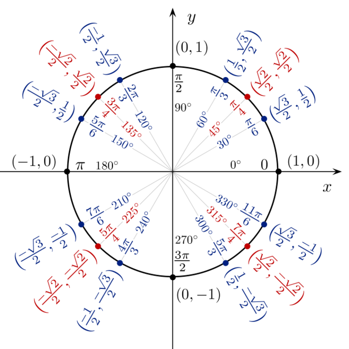
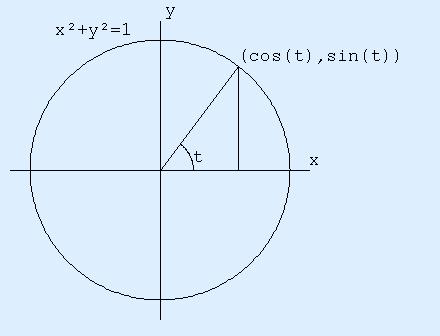
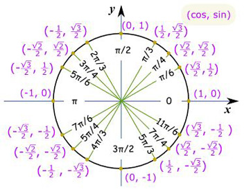
In the unit circle:

sin θ represents the y-coordinate
cos θ represents the x-coordinate
tan θ represents y/x

Understanding these relationships helps in solving trigonometric equations.


Periodicity of Trigonometric Functions

Image
Image
Image
Image

One of the most important properties of trigonometric functions is periodicity.

A periodic function repeats its values after a fixed interval called the period.

Period of Sine and Cosine

The period of sine and cosine functions is:

360° or 2π radians

This means:

sin(x + 360°) = sin x
cos(x + 360°) = cos x

Period of Tangent

The tangent function has a smaller period:

180° or π radians

tan(x + 180°) = tan x

Because of periodicity, trigonometric equations usually have infinitely many solutions.

For example:

sin x = 0

Solutions include:

0°, 180°, 360°, 540°, and so on.

General solution:

x = nπ

where n is an integer.


Types of Trigonometric Equations

Trigonometric equations can appear in many different forms.

Common types include:

  1. Basic trigonometric equations
  2. Linear trigonometric equations
  3. Quadratic trigonometric equations
  4. Multiple-angle equations
  5. Equations involving identities
  6. Equations with inverse trigonometric functions

Each type requires different solving strategies.


Solving Basic Trigonometric Equations

Image
Image
Image
Image

Basic trigonometric equations involve a single trigonometric function.

Example:

sin x = 1/2

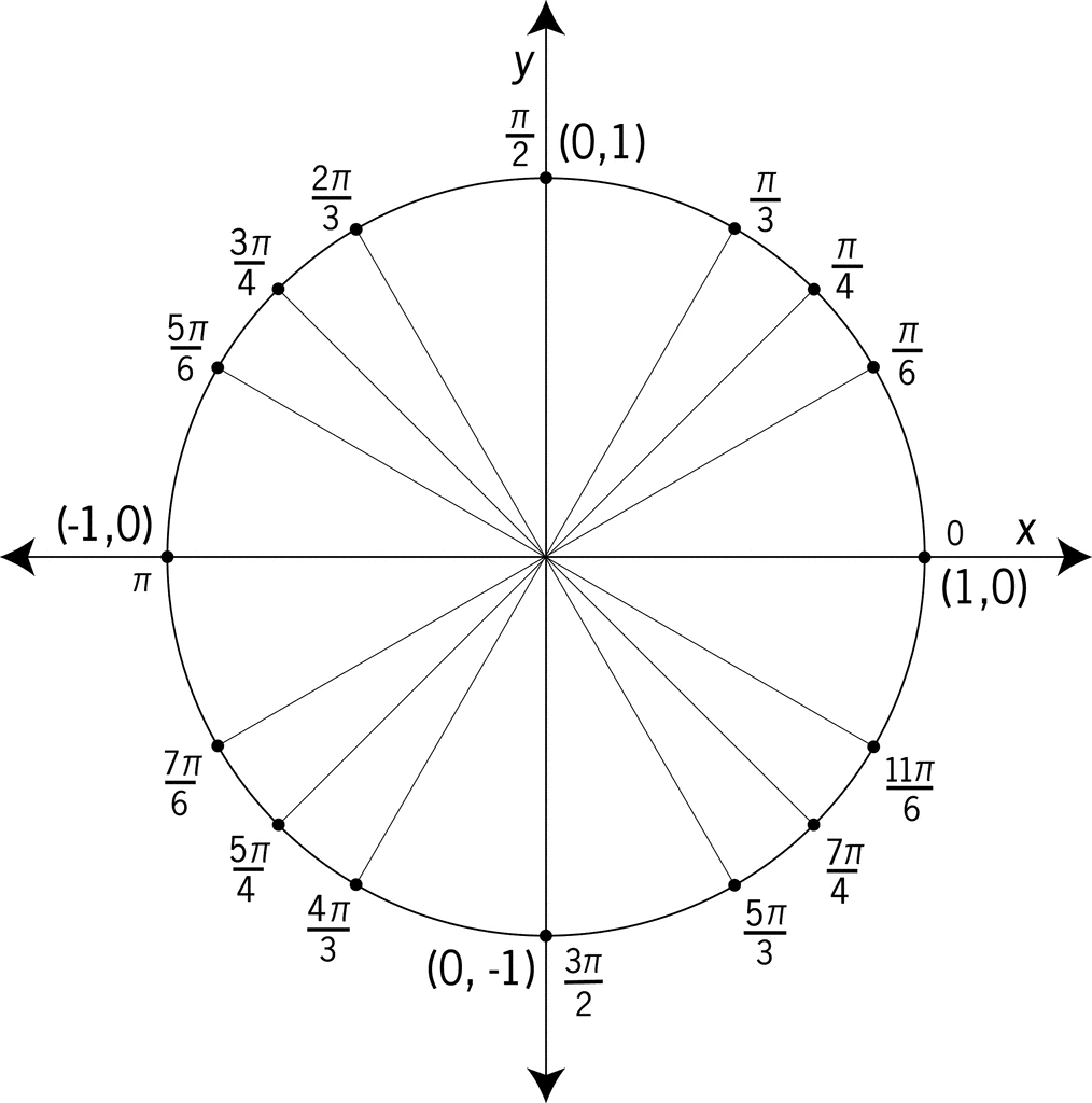
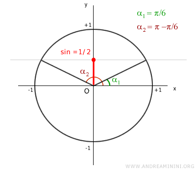
Using the unit circle:

sin 30° = 1/2
sin 150° = 1/2

Therefore:

x = 30° or 150°

General solution:

x = 30° + 360°n
x = 150° + 360°n

where n is an integer.

Another example:

cos x = 0

From the unit circle:

cos 90° = 0
cos 270° = 0

General solution:

x = 90° + 180°n


Solving Trigonometric Equations Using Identities

Image
Image
Image
Image

Many trigonometric equations require the use of identities.

Important identities include:

sin²x + cos²x = 1
1 + tan²x = sec²x
1 + cot²x = csc²x

Example:

sin²x + cos²x = 1

This identity is always true.

Example equation:

sin²x = 1 − cos²x

This identity can simplify equations.

Example:

2sin²x − 1 = 0

Add 1:

2sin²x = 1

Divide by 2:

sin²x = 1/2

Take square root:

sin x = ± √2/2

Solutions:

x = 45°, 135°, 225°, 315°


Quadratic Trigonometric Equations

Image
Image
Image
Image

Some trigonometric equations behave like quadratic equations.

Example:

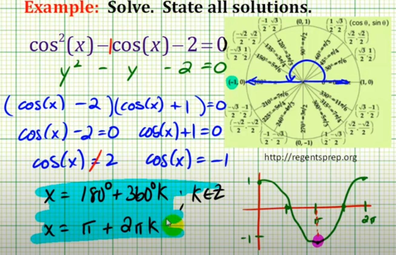
2sin²x − 3sin x + 1 = 0

Let:

sin x = y

Then equation becomes:

2y² − 3y + 1 = 0

Factor:

(2y − 1)(y − 1) = 0

Solutions:

y = 1/2
y = 1

Therefore:

sin x = 1/2
sin x = 1

Using the unit circle:

sin x = 1/2 → x = 30°, 150°

sin x = 1 → x = 90°

Thus solutions include:

30°, 90°, 150°


Trigonometric Equations with Multiple Angles

Image
Image
Image
Image

Some equations involve multiple angles such as 2x or 3x.

Example:

sin(2x) = √3/2

From the unit circle:

2x = 60° or 120°

Divide by 2:

x = 30° or 60°

General solution:

x = 30° + 180°n
x = 60° + 180°n

These equations often require double-angle or triple-angle identities.

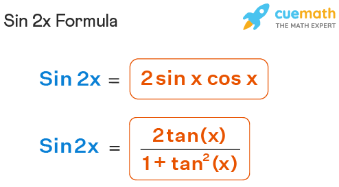
Example identity:

sin(2x) = 2sin x cos x


Graphical Method for Solving Trigonometric Equations

Image
Image
Image
Image

Trigonometric equations can also be solved graphically.

Example:

sin x = cos x

Rewrite:

tan x = 1

From unit circle:

x = 45°, 225°

Graphically, the solutions correspond to the intersection points of the graphs of sin x and cos x.

Graphing methods are especially useful when equations are complicated.


Inverse Trigonometric Functions in Equations

Image
Image
Image
Image

Inverse trigonometric functions help solve equations where the angle is unknown.

Example:

sin x = 0.8

Use inverse sine:

x = sin⁻¹(0.8)

x ≈ 53.13°

Because sine is positive in the first and second quadrants:

x = 53.13°
x = 180° − 53.13° = 126.87°

General solution:

x = 53.13° + 360°n
x = 126.87° + 360°n


Applications of Trigonometric Equations

Trigonometric equations are widely used in real-world applications.

Physics

They are used to analyze:

  • wave motion
  • harmonic oscillations
  • light waves
  • sound waves

Engineering

Engineers use trigonometric equations for:

  • signal processing
  • electrical circuits
  • mechanical vibrations
  • structural analysis

Astronomy

Astronomers use trigonometry to determine:

  • distances between stars
  • orbital motion of planets
  • angles between celestial objects

Navigation

Trigonometry helps in:

  • aircraft navigation
  • GPS positioning
  • ship navigation

Computer Graphics

3D modeling and animation depend heavily on trigonometric equations for rotations and transformations.


Importance of Trigonometric Equations in Mathematics

Trigonometric equations are fundamental to advanced mathematics.

They are essential in:

  • calculus
  • differential equations
  • Fourier analysis
  • complex numbers
  • signal processing

They help model periodic patterns found in nature and technology.

Understanding how to solve trigonometric equations strengthens algebraic reasoning and mathematical problem-solving skills.


Conclusion

Trigonometric equations are equations that involve trigonometric functions and require determining the angles that satisfy the equation. Because trigonometric functions are periodic, these equations often have infinitely many solutions.

Solving trigonometric equations requires knowledge of trigonometric identities, unit circle values, algebraic techniques, and inverse trigonometric functions. Different types of equations require different strategies, such as factoring, identity substitution, graphical analysis, or inverse functions.

These equations play a crucial role in mathematics, physics, engineering, astronomy, and computer science. Mastering trigonometric equations provides a strong foundation for advanced mathematical studies and real-world applications involving periodic behavior.


Tags

Trigonometric Identities

Image
Image
Image
Image

Introduction to Trigonometric Identities

Trigonometric identities are mathematical equations that involve trigonometric functions and remain true for all values of the variables for which the functions are defined. These identities are essential tools in mathematics because they allow us to simplify complex trigonometric expressions, solve trigonometric equations, prove relationships between functions, and analyze periodic phenomena in science and engineering.

The primary trigonometric functions involved in identities include:

  • sine (sin)
  • cosine (cos)
  • tangent (tan)
  • cosecant (csc)
  • secant (sec)
  • cotangent (cot)

These functions are interrelated through various identities that arise from geometric properties of right triangles and the unit circle.

Trigonometric identities are widely used in algebra, geometry, calculus, physics, engineering, signal processing, astronomy, and many other scientific disciplines. Understanding these identities enables mathematicians and scientists to manipulate trigonometric expressions efficiently and solve problems involving angles and periodic motion.


Basic Trigonometric Functions

Image
Image
Image
Image

Before studying trigonometric identities, it is important to understand the six trigonometric functions.

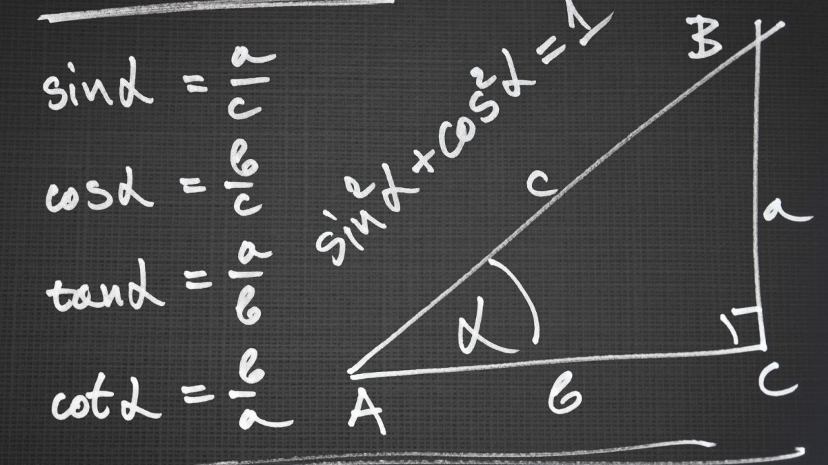
In a right triangle:

  • sin θ = opposite / hypotenuse
  • cos θ = adjacent / hypotenuse
  • tan θ = opposite / adjacent

The reciprocal functions are:

  • csc θ = 1 / sin θ
  • sec θ = 1 / cos θ
  • cot θ = 1 / tan θ

These functions are the foundation of trigonometric identities.

For example:

If the opposite side is 3, adjacent side is 4, and hypotenuse is 5:

sin θ = 3/5
cos θ = 4/5
tan θ = 3/4

Using reciprocals:

csc θ = 5/3
sec θ = 5/4
cot θ = 4/3

These relationships allow the formation of many identities.


Types of Trigonometric Identities

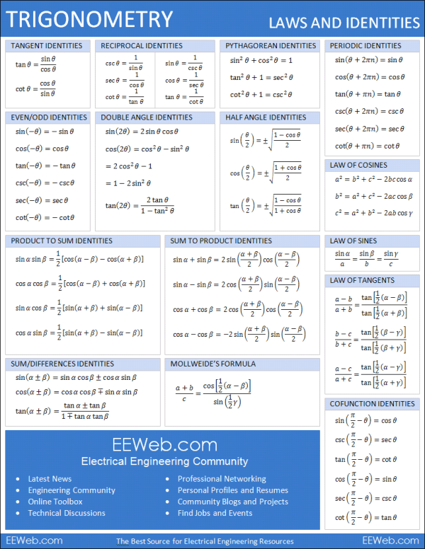
Trigonometric identities are generally classified into several categories:

  1. Reciprocal identities
  2. Quotient identities
  3. Pythagorean identities
  4. Co-function identities
  5. Even and odd identities
  6. Sum and difference identities
  7. Double angle identities
  8. Half-angle identities
  9. Product-to-sum identities

Each group of identities plays an important role in mathematical problem solving.


Reciprocal Identities

Image
Image
Image
Image

Reciprocal identities show the relationship between a trigonometric function and its reciprocal.

The identities are:

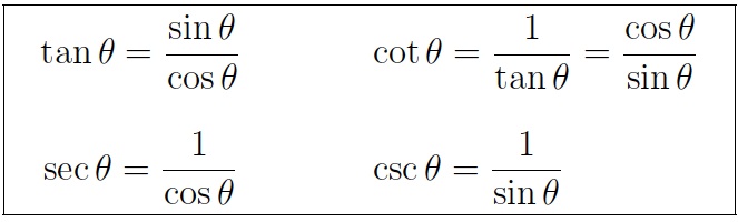
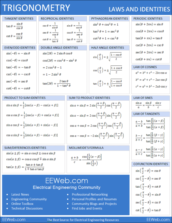
csc θ = 1 / sin θ
sec θ = 1 / cos θ
cot θ = 1 / tan θ

Similarly,

sin θ = 1 / csc θ
cos θ = 1 / sec θ
tan θ = 1 / cot θ

These identities arise from the reciprocal nature of the trigonometric functions.

Example

If

sin θ = 1/2

Then

csc θ = 2

Because

csc θ = 1 / sin θ

Reciprocal identities are often used to rewrite expressions in different forms.


Quotient Identities

Image
Image
Image
Image

Quotient identities relate tangent and cotangent to sine and cosine.

The identities are:

tan θ = sin θ / cos θ

cot θ = cos θ / sin θ

These identities come directly from the definitions of trigonometric ratios.

Example

If

sin θ = 0.6
cos θ = 0.8

Then

tan θ = 0.6 / 0.8 = 0.75

Quotient identities are useful when converting expressions between trigonometric forms.


Pythagorean Identities

Image
Image
Image
Image

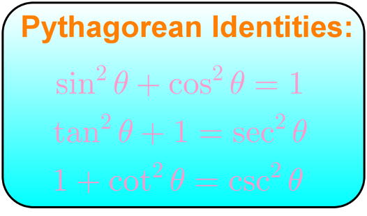
Pythagorean identities are derived from the Pythagorean theorem.

In a right triangle:

a² + b² = c²

Using trigonometric ratios, this relationship leads to the fundamental identity:

sin² θ + cos² θ = 1

Other identities derived from this include:

1 + tan² θ = sec² θ

1 + cot² θ = csc² θ

Derivation

Divide the Pythagorean equation by hypotenuse².

(opposite/hypotenuse)² + (adjacent/hypotenuse)² = 1

This gives:

sin² θ + cos² θ = 1

Example

If

sin θ = 0.6

Then

sin² θ = 0.36

Using identity:

cos² θ = 1 − 0.36 = 0.64

cos θ = 0.8

These identities are extremely important in simplifying trigonometric expressions.


Co-Function Identities

Image
Image
Image
Image

Co-function identities describe relationships between trigonometric functions of complementary angles.

Complementary angles add up to 90°.

The identities are:

sin(90° − θ) = cos θ

cos(90° − θ) = sin θ

tan(90° − θ) = cot θ

cot(90° − θ) = tan θ

sec(90° − θ) = csc θ

csc(90° − θ) = sec θ

These identities arise from the geometry of right triangles.

Example

sin(90° − 30°)

sin(60°)

Which equals

√3 / 2

Thus

cos 30° = sin 60°


Even and Odd Identities

Image
Image
Image
Image

Some trigonometric functions are even, while others are odd.

Even Functions

cos(−θ) = cos θ
sec(−θ) = sec θ

Even functions are symmetric about the y-axis.

Odd Functions

sin(−θ) = −sin θ

tan(−θ) = −tan θ

cot(−θ) = −cot θ

csc(−θ) = −csc θ

Odd functions are symmetric about the origin.

These identities are useful in simplifying expressions involving negative angles.


Sum and Difference Identities

Image
Image
Image
Image

Sum and difference identities express trigonometric functions of sums or differences of angles.

Sine

sin(A + B) = sinA cosB + cosA sinB

sin(A − B) = sinA cosB − cosA sinB

Cosine

cos(A + B) = cosA cosB − sinA sinB

cos(A − B) = cosA cosB + sinA sinB

Tangent

tan(A + B) = (tanA + tanB) / (1 − tanA tanB)

tan(A − B) = (tanA − tanB) / (1 + tanA tanB)

These formulas are important for solving trigonometric equations and simplifying expressions.


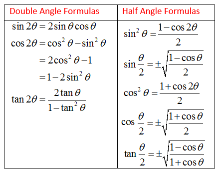
Double Angle Identities

Image
Image
Image
Image

Double angle identities express trigonometric functions of twice an angle.

Sine

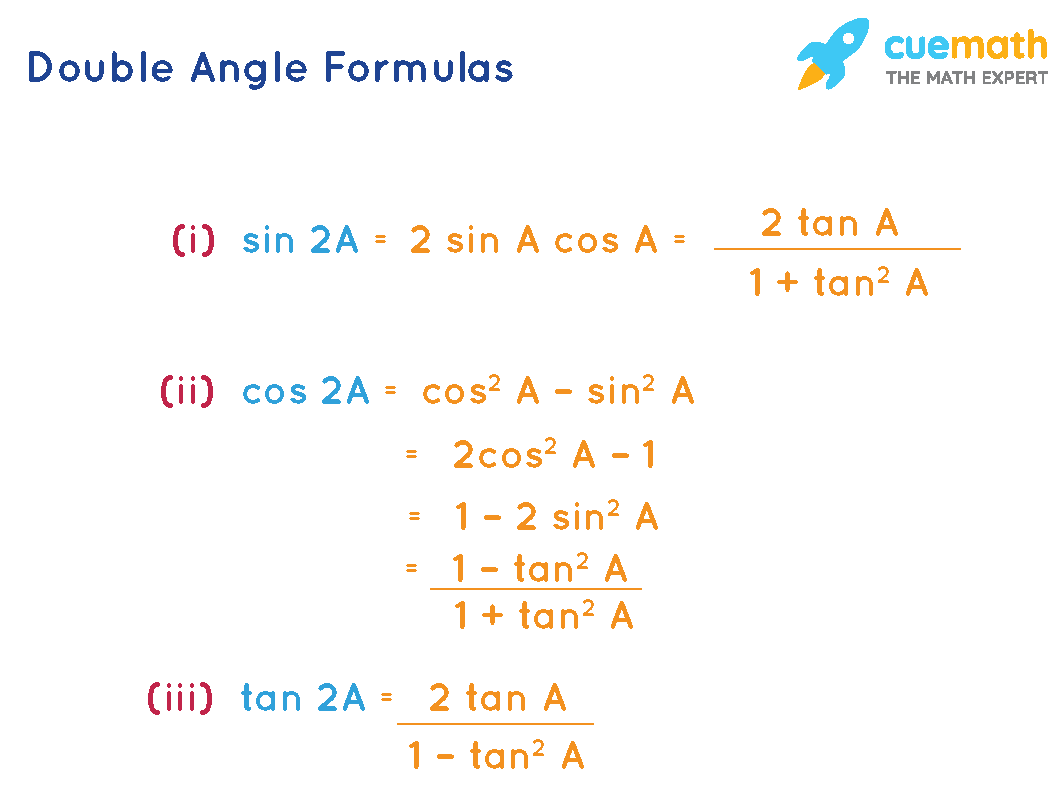
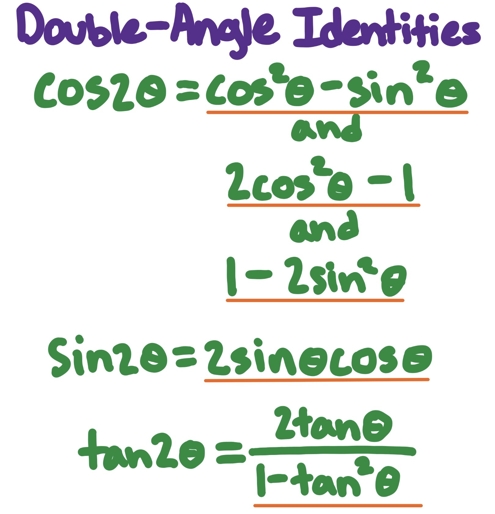
sin(2θ) = 2 sinθ cosθ

Cosine

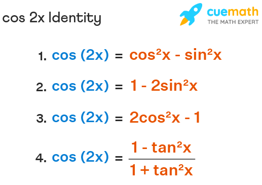
cos(2θ) = cos²θ − sin²θ

This identity can also be written as:

cos(2θ) = 2cos²θ − 1

cos(2θ) = 1 − 2sin²θ

Tangent

tan(2θ) = (2tanθ) / (1 − tan²θ)

These identities are used extensively in calculus and physics.


Half-Angle Identities

Image
Image
Image
Image

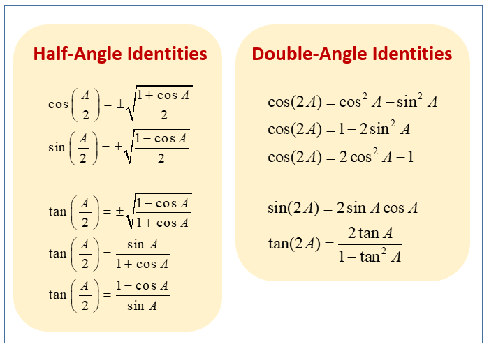
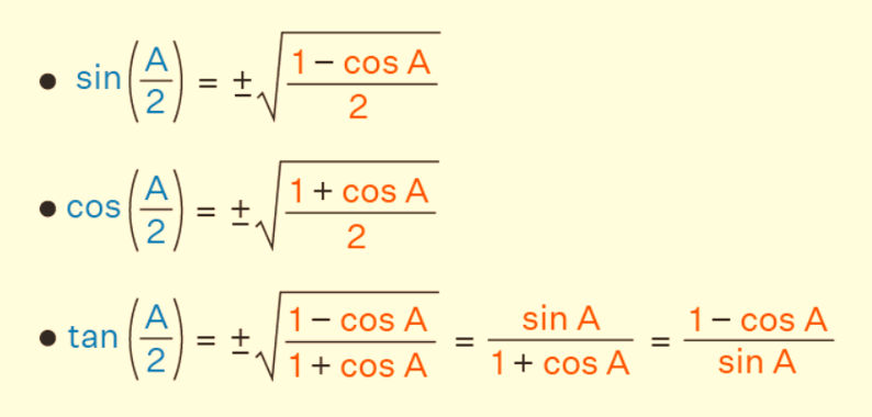
Half-angle identities express trigonometric functions of half an angle.

sin(θ/2) = √((1 − cosθ)/2)

cos(θ/2) = √((1 + cosθ)/2)

tan(θ/2) = (1 − cosθ)/sinθ

These identities are useful in calculus, integration, and solving trigonometric equations.


Product-to-Sum Identities

Image
Image
Image
Image

Product-to-sum identities convert products of trigonometric functions into sums.

Examples:

sinA sinB = ½ [cos(A − B) − cos(A + B)]

cosA cosB = ½ [cos(A − B) + cos(A + B)]

sinA cosB = ½ [sin(A + B) + sin(A − B)]

These identities are useful in signal processing and wave analysis.


Applications of Trigonometric Identities

Trigonometric identities are widely used in many areas of science and engineering.

Physics

They are used to study:

  • wave motion
  • sound waves
  • light waves
  • alternating current circuits

Engineering

Engineers use trigonometric identities in:

  • structural analysis
  • mechanical systems
  • robotics
  • electrical engineering

Astronomy

Astronomers apply trigonometry to determine:

  • planetary motion
  • distance between celestial objects
  • orbital paths

Computer Graphics

3D modeling and animation rely heavily on trigonometric identities to compute rotations, transformations, and rendering.

Navigation

Trigonometry helps determine distances and directions for aircraft, ships, and satellites.


Importance of Trigonometric Identities in Mathematics

Trigonometric identities play a crucial role in advanced mathematics.

They are essential in:

  • calculus
  • differential equations
  • Fourier series
  • complex numbers
  • signal processing

They help simplify complicated expressions and solve equations that would otherwise be extremely difficult.


Conclusion

Trigonometric identities are fundamental relationships between trigonometric functions that remain true for all valid values of the variables. These identities arise from the geometric properties of triangles and the unit circle and provide powerful tools for solving mathematical problems.

The major categories of trigonometric identities include reciprocal identities, quotient identities, Pythagorean identities, co-function identities, sum and difference identities, double-angle identities, half-angle identities, and product-to-sum identities. Each group of identities serves a specific purpose in simplifying expressions and solving equations.

Understanding trigonometric identities is essential for students studying mathematics, physics, engineering, and many other scientific disciplines. Mastery of these identities enables efficient problem solving and provides a deeper understanding of the relationships between angles, functions, and periodic phenomena.


Tags

Trigonometric Ratios (Sin, Cos, Tan)

Image
Image
Image
Image

Introduction to Trigonometric Ratios

Trigonometry is a branch of mathematics that studies the relationships between the angles and sides of triangles. The word trigonometry originates from the Greek words trigonon (triangle) and metron (measure). It plays a fundamental role in many fields such as physics, engineering, architecture, navigation, astronomy, computer graphics, and even modern technologies like satellite communication and robotics.

Among the many concepts in trigonometry, trigonometric ratios are the most fundamental. These ratios describe the relationship between the angles of a right triangle and the lengths of its sides. The three primary trigonometric ratios are:

  • Sine (sin)
  • Cosine (cos)
  • Tangent (tan)

These ratios allow us to determine unknown sides or angles of a triangle when some information is known.

Trigonometric ratios are primarily defined using a right-angled triangle, which is a triangle containing one angle equal to 90°. In such a triangle, the sides are classified based on the reference angle (the angle we are considering).

Parts of a Right Triangle

A right triangle consists of three sides:

  1. Hypotenuse
  2. Opposite side
  3. Adjacent side

The hypotenuse is the longest side and lies opposite the right angle. The other two sides are defined relative to the chosen angle.

  • Opposite side: The side opposite the reference angle.
  • Adjacent side: The side next to the reference angle but not the hypotenuse.

These definitions help in forming the trigonometric ratios.


Understanding Sine (sin)

Image
Image
Image

Definition of Sine

The sine of an angle in a right triangle is defined as the ratio of the length of the opposite side to the length of the hypotenuse.

Mathematically,

[
\sin(\theta) = \frac{\text{Opposite}}{\text{Hypotenuse}}
]

Where:

  • θ represents the angle
  • Opposite is the side opposite the angle
  • Hypotenuse is the longest side of the triangle

Example

Suppose in a right triangle:

Opposite side = 4
Hypotenuse = 5

[
\sin(\theta) = \frac{4}{5} = 0.8
]

This means the sine of angle θ equals 0.8.

Interpretation

The sine ratio represents how much the triangle rises vertically compared to the hypotenuse. In geometric terms, it measures the vertical component of an angle.

Sine in the Unit Circle

In the unit circle, which is a circle of radius 1 centered at the origin, sine represents the y-coordinate of a point corresponding to an angle.

For example:

  • sin(0°) = 0
  • sin(30°) = 0.5
  • sin(90°) = 1

Important Sine Values

AngleSin Value
0
30°1/2
45°√2/2
60°√3/2
90°1

These values are commonly used in trigonometric calculations.

Properties of Sine

  1. Range of sine values: -1 ≤ sinθ ≤ 1
  2. Periodic function with period 360°
  3. Positive in the first and second quadrants
  4. Negative in the third and fourth quadrants

Applications of Sine

Sine is widely used in various real-world applications:

  • Calculating heights of buildings
  • Studying wave motion in physics
  • Sound and light wave analysis
  • Electrical engineering (AC circuits)
  • Astronomy and satellite motion

Understanding Cosine (cos)

Image
Image
Image

Definition of Cosine

The cosine of an angle in a right triangle is defined as the ratio of the adjacent side to the hypotenuse.

[
\cos(\theta) = \frac{\text{Adjacent}}{\text{Hypotenuse}}
]

Where:

  • Adjacent is the side next to the angle
  • Hypotenuse is the longest side

Example

Adjacent side = 3
Hypotenuse = 5

[
\cos(\theta) = \frac{3}{5} = 0.6
]

Interpretation

Cosine represents the horizontal component of an angle. It measures how much the triangle extends horizontally compared to the hypotenuse.

Cosine in the Unit Circle

In the unit circle, cosine represents the x-coordinate of the point corresponding to an angle.

Examples:

  • cos(0°) = 1
  • cos(60°) = 0.5
  • cos(90°) = 0

Important Cosine Values

AngleCos Value
1
30°√3/2
45°√2/2
60°1/2
90°0

Properties of Cosine

  1. Range: -1 ≤ cosθ ≤ 1
  2. Period: 360°
  3. Positive in the first and fourth quadrants
  4. Negative in the second and third quadrants

Cosine in Physics

Cosine is extremely important in physics because it is used in:

  • Force components
  • Motion analysis
  • Vector calculations
  • Wave mechanics
  • Signal processing

For example, if a force is applied at an angle, cosine helps determine the horizontal component of the force.


Understanding Tangent (tan)

Image
Image
Image
Image

Definition of Tangent

The tangent of an angle in a right triangle is defined as the ratio of the opposite side to the adjacent side.

[
\tan(\theta) = \frac{\text{Opposite}}{\text{Adjacent}}
]

Example

Opposite side = 4
Adjacent side = 3

[
\tan(\theta) = \frac{4}{3}
]

Relationship with Sine and Cosine

Tangent can also be expressed as:

[
\tan(\theta) = \frac{\sin(\theta)}{\cos(\theta)}
]

This relationship is extremely important in trigonometry.

Important Tangent Values

AngleTan Value
0
30°1/√3
45°1
60°√3
90°Undefined

Tangent becomes undefined at 90° because cosine becomes zero.

Properties of Tangent

  1. Range: −∞ to +∞
  2. Period: 180°
  3. Positive in first and third quadrants
  4. Negative in second and fourth quadrants

Applications of Tangent

Tangent is commonly used to calculate:

  • Heights of mountains
  • Distance of objects
  • Slopes in engineering
  • Angles of elevation and depression

For example, if you know the distance from a building and the angle of elevation, tangent can help calculate the height.


Relationship Between Sin, Cos, and Tan

Trigonometric ratios are interconnected through several identities.

Pythagorean Identity

One of the most important identities is:

[
\sin^2(\theta) + \cos^2(\theta) = 1
]

This identity comes from the Pythagorean theorem.

Tangent Identity

[
\tan(\theta) = \frac{\sin(\theta)}{\cos(\theta)}
]

Reciprocal Relationships

Although sin, cos, and tan are primary ratios, there are also reciprocal ratios:

  • cosec = 1/sin
  • sec = 1/cos
  • cot = 1/tan

Trigonometric Ratios in Different Quadrants

The coordinate plane is divided into four quadrants.

QuadrantSign of sinSign of cosSign of tan
I+++
II+
III+
IV+

A helpful mnemonic to remember this is:

ASTC (All Students Take Calculus)

  • Quadrant 1: All positive
  • Quadrant 2: Sine positive
  • Quadrant 3: Tangent positive
  • Quadrant 4: Cosine positive

Angles of Elevation and Depression

Trigonometric ratios are used to solve real-life problems involving heights and distances.

Angle of Elevation

The angle between the horizontal line and the line of sight when looking upwards.

Example:

If a person stands 20 meters from a building and the angle of elevation to the top is 45°:

[
\tan(45°) = \frac{Height}{20}
]

Since tan45° = 1

Height = 20 meters

Angle of Depression

The angle between the horizontal line and the line of sight when looking downwards.

These concepts are widely used in surveying and navigation.


Trigonometric Functions Graphs

Sine Graph

The sine graph is a smooth wave that oscillates between -1 and 1.

Key characteristics:

  • Period = 360°
  • Amplitude = 1
  • Starts at 0

Cosine Graph

The cosine graph also oscillates between -1 and 1 but starts at 1 when angle = 0°.

Tangent Graph

The tangent graph has vertical asymptotes and repeats every 180°.


Real-World Applications of Trigonometric Ratios

Trigonometry is widely used in science and technology.

Architecture

Architects use trigonometry to determine:

  • Structural angles
  • Roof slopes
  • Building heights

Navigation

Trigonometry helps in:

  • Calculating distances between locations
  • Satellite navigation
  • GPS technology

Engineering

Engineers apply trigonometry in:

  • Bridge design
  • Mechanical systems
  • Electrical signal analysis

Astronomy

Astronomers use trigonometric calculations to measure:

  • Distance between planets
  • Position of stars
  • Orbital motion

Computer Graphics

3D modeling and animation rely heavily on trigonometric functions to calculate angles and rotations.


Solving Right Triangles Using Trigonometric Ratios

Trigonometric ratios allow us to solve triangles when some information is known.

Example problem:

Given:

Hypotenuse = 10
Angle = 30°

Find opposite side.

[
\sin(30°) = \frac{Opposite}{10}
]

[
\frac{1}{2} = \frac{Opposite}{10}
]

Opposite = 5

Thus, the opposite side equals 5 units.


Importance of Trigonometric Ratios in Mathematics

Trigonometric ratios serve as the foundation for many advanced mathematical concepts such as:

  • Trigonometric identities
  • Calculus
  • Fourier analysis
  • Differential equations
  • Vector mathematics

They also help students develop strong problem-solving skills and spatial reasoning.


Summary

Trigonometric ratios are essential tools in mathematics that describe relationships between angles and sides of triangles. The three main ratios are:

  • Sine (sin): Opposite / Hypotenuse
  • Cosine (cos): Adjacent / Hypotenuse
  • Tangent (tan): Opposite / Adjacent

These ratios are interconnected through identities and play a crucial role in solving geometric problems involving triangles. They are widely applied in science, engineering, architecture, navigation, and technology.

Understanding trigonometric ratios provides the foundation for more advanced studies in mathematics and enables practical problem solving in real-world situations.
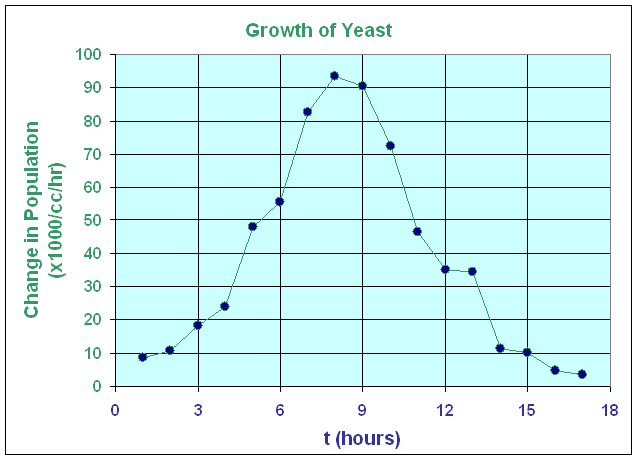

Tags