

Tags:
1. Introduction to Linear Algebra
Linear Algebra is one of the fundamental branches of mathematics that deals with vectors, vector spaces, matrices, and linear transformations. It forms the mathematical backbone of many scientific and engineering disciplines including physics, computer science, artificial intelligence, data science, economics, and engineering.
At its core, Linear Algebra studies linear relationships between variables. A relationship is linear if it satisfies the properties of additivity and homogeneity, meaning the function behaves predictably under addition and scalar multiplication.
Historically, Linear Algebra evolved from solving systems of linear equations. Ancient civilizations such as the Chinese used matrix-like methods in texts like The Nine Chapters on the Mathematical Art. Later, mathematicians such as Carl Friedrich Gauss and Augustin-Louis Cauchy developed systematic techniques that led to modern matrix theory.
Today, Linear Algebra plays a central role in computational mathematics, machine learning, robotics, computer graphics, and quantum mechanics.
2. Systems of Linear Equations
A linear equation is an equation where each variable appears only to the first power and variables are not multiplied together.
Example:
2x + 3y = 5
x - y = 2
A system of linear equations consists of multiple linear equations involving the same variables.
Example:
2x + y + z = 4
x + 3y - z = 5
3x - y + 2z = 6
The goal is to find values of variables that satisfy all equations simultaneously.
Types of Solutions
- Unique solution – exactly one solution.
- Infinite solutions – infinitely many solutions.
- No solution – inconsistent system.
Methods to Solve Systems
Substitution Method
One equation is solved for one variable and substituted into another.
Elimination Method
Variables are eliminated through addition or subtraction.
Gaussian Elimination
Transforms equations into an upper triangular form.
Gauss–Jordan Elimination
Transforms the matrix into Reduced Row Echelon Form (RREF).
Example matrix representation:
[2 3 | 5]
[1 -1 | 2]
This method allows efficient computational solving of large systems.
3. Matrices
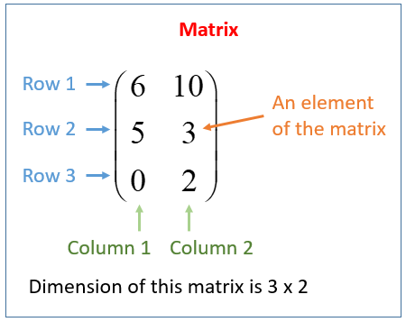

A matrix is a rectangular arrangement of numbers organized in rows and columns.
Example:
A = [ 2 4
      1 3 ]
If a matrix has m rows and n columns, it is called an m × n matrix.
Types of Matrices
- Row Matrix
One row. - Column Matrix
One column. - Square Matrix
Equal rows and columns. - Zero Matrix
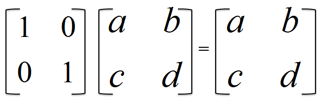
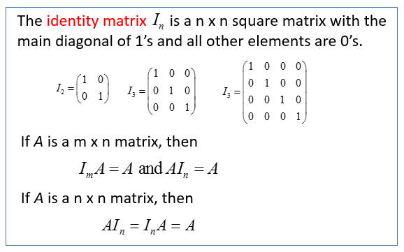
All elements are zero. - Identity Matrix
I =
[1 0
 0 1]
- Diagonal Matrix
[5 0 0
 0 3 0
 0 0 1]
- Symmetric Matrix
A = Aᵀ
Matrix Operations
Matrix Addition
Two matrices of the same size can be added.
A + B = [a_ij + b_ij]
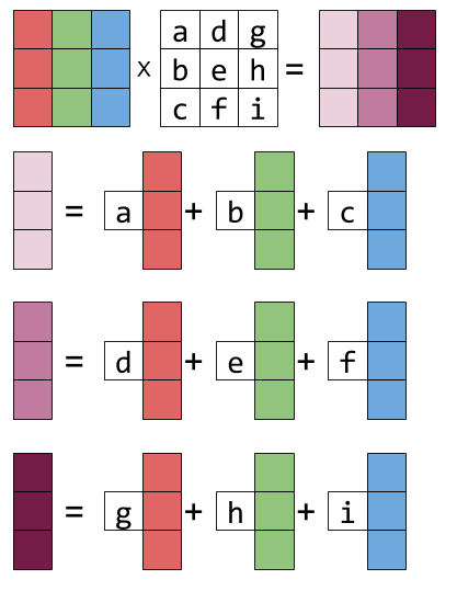
Matrix Multiplication
If A is m × n and B is n × p, the product AB is m × p.
Example:
A = [1 2]
    [3 4]

B = [5 6]
    [7 8]
AB = [19 22
      43 50]
Matrix multiplication is not commutative.
AB ≠ BA
Transpose of a Matrix
The transpose swaps rows and columns.
Aᵀ
Example:
A =
[1 2 3
 4 5 6]

Aᵀ =
[1 4
 2 5
 3 6]
4. Determinants


A determinant is a scalar value associated with a square matrix. It provides important information about the matrix, including:
- Whether a matrix is invertible
- Scaling factor of linear transformations
- Volume transformation
For a 2×2 matrix:
|a b|
|c d|
Determinant:
ad − bc
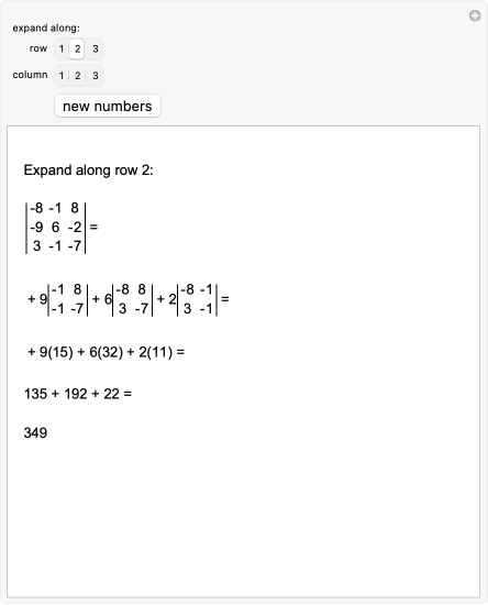
For a 3×3 matrix:
|a b c|
|d e f|
|g h i|
Determinant:
a(ei − fh) − b(di − fg) + c(dh − eg)
Properties of Determinants
- det(Aᵀ) = det(A)
- det(AB) = det(A)det(B)
- det(I) = 1
- If two rows are equal → determinant = 0
A matrix is invertible if determinant ≠ 0.
5. Vectors
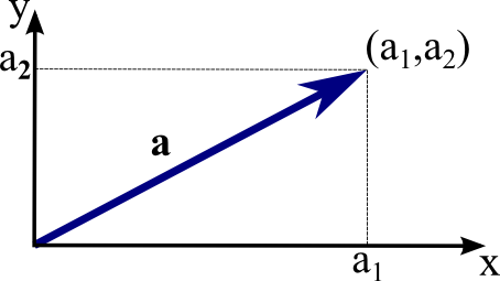


A vector represents both magnitude and direction.
Example in 2D:
v = (3,4)
Vector Operations
Vector Addition
(1,2) + (3,4) = (4,6)
Scalar Multiplication
2(1,3) = (2,6)
Dot Product
a · b = |a||b|cosθ
Example:
(1,2) · (3,4) = 11
Applications:
- Finding angles
- Projections
- Orthogonality
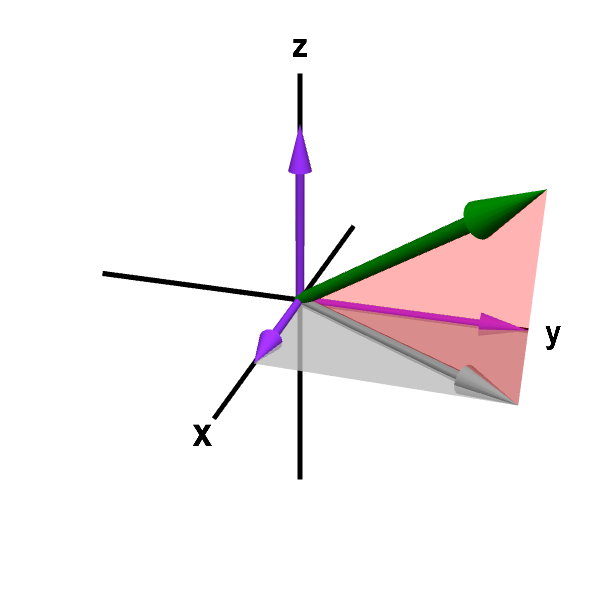
Cross Product
In 3D:
a × b
Produces a vector perpendicular to both vectors.
6. Vector Spaces
A vector space is a collection of vectors that satisfy certain rules.
Examples:
- ℝ²
- ℝ³
- Polynomial spaces
- Function spaces
Vector Space Axioms
Key properties include:
- Closure under addition
- Closure under scalar multiplication
- Existence of zero vector
- Existence of additive inverse
- Associativity
- Distributive properties
Subspaces
A subset of a vector space that is itself a vector space.
Conditions:
- Contains zero vector
- Closed under addition
- Closed under scalar multiplication
Example:
The set of vectors on a plane in 3D space.
7. Basis and Dimension
A basis is a set of linearly independent vectors that span a vector space.
Example in ℝ²:
(1,0)
(0,1)
These vectors form the standard basis.
Dimension
The number of vectors in a basis.
Examples:
- ℝ² → dimension = 2
- ℝ³ → dimension = 3
8. Linear Independence
Vectors are linearly independent if none can be written as a combination of others.
Example:
(1,0)
(0,1)
Independent.
Example of dependence:
(1,2)
(2,4)
Second vector is a multiple of the first.
Mathematically:
c1v1 + c2v2 + ... + cnvn = 0
If the only solution is:
c1 = c2 = ... = 0
then vectors are independent.
9. Linear Transformations

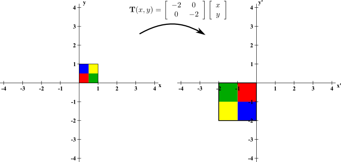
A linear transformation is a function between vector spaces preserving linearity.
If T is linear:
T(u + v) = T(u) + T(v)
T(cv) = cT(v)
Example:
Rotation in 2D.
Matrix representation:
T(x) = Ax
Example matrix:
[0 -1
 1  0]
This rotates vectors by 90°.
10. Eigenvalues and Eigenvectors


An eigenvector of a matrix is a vector whose direction does not change after transformation.
Mathematically:
Av = λv
Where:
- A = matrix
- v = eigenvector
- λ = eigenvalue
Finding Eigenvalues
Solve:
det(A − λI) = 0
This is called the characteristic equation.
Example uses:
- Google PageRank
- PCA in machine learning
- Quantum mechanics
11. Orthogonality
Vectors are orthogonal if their dot product equals zero.
a · b = 0
Orthogonal vectors are perpendicular.
Orthonormal Basis
Vectors that are:
- Orthogonal
- Unit length
Example:
(1,0)
(0,1)
12. Matrix Decompositions
Important decompositions include:
LU Decomposition
A = LU
Where:
- L = Lower triangular
- U = Upper triangular
QR Decomposition
A = QR
Where:
- Q = Orthogonal matrix
- R = Upper triangular matrix
Singular Value Decomposition (SVD)
A = UΣVᵀ
Applications:
- Data compression
- Image processing
- Recommendation systems
13. Applications of Linear Algebra
Linear Algebra is used in many fields.
Computer Graphics
3D transformations:
- rotation
- scaling
- translation
Used in gaming engines and animation.
Machine Learning
Algorithms use matrices and vectors:
- Neural networks
- PCA
- Linear regression
Data Science
Used for:
- dimensionality reduction
- recommendation systems
- clustering
Physics
Quantum mechanics uses Hilbert spaces and linear operators.
Engineering
Used in:
- electrical circuits
- signal processing
- control systems
Economics
Input-output models of industries use matrices.
14. Linear Algebra in Artificial Intelligence
Modern AI relies heavily on Linear Algebra.
Neural networks are built using:
- matrix multiplications
- vector operations
- gradient calculations
Example neural network layer:
y = Wx + b
Where:
- W = weight matrix
- x = input vector
- b = bias vector
Training algorithms use gradient descent, which also depends on vector calculus and matrix operations.
15. Computational Linear Algebra
Large datasets require efficient algorithms.
Popular numerical techniques include:
- Iterative solvers
- Sparse matrix methods
- Krylov subspace methods
Libraries used in computing:
- BLAS
- LAPACK
- NumPy
These allow efficient matrix operations in scientific computing.
16. Advanced Topics
Advanced concepts include:
Tensor Algebra
Generalization of matrices to higher dimensions.
Spectral Theory
Study of eigenvalues of operators.
Functional Analysis
Extends linear algebra to infinite-dimensional spaces.
Numerical Linear Algebra
Focuses on stable algorithms for computers.
17. Importance of Linear Algebra
Linear Algebra is considered one of the most important mathematical tools because:
- It simplifies complex systems.
- It provides geometric insight into equations.
- It enables efficient computation.
- It forms the basis of modern technology.
Fields like AI, robotics, data science, and physics would not exist in their current form without linear algebra.
18. Summary
Linear Algebra studies mathematical structures that model linear relationships. Core components include:
- vectors
- matrices
- vector spaces
- determinants
- eigenvalues
- linear transformations
These concepts allow scientists and engineers to represent and solve complex real-world problems.
From solving systems of equations to powering artificial intelligence algorithms, Linear Algebra remains a foundational pillar of modern mathematics and technology.