


Introduction to Probability Distributions
Probability distributions are fundamental concepts in probability theory and statistics that describe how the values of a random variable are distributed across possible outcomes. In many real-world situations, outcomes of events are uncertain, and probability distributions help quantify and analyze this uncertainty.
A probability distribution provides a mathematical function that gives the probability of occurrence of different possible outcomes of a random variable. In simple terms, it shows how likely each value of a variable is to occur.
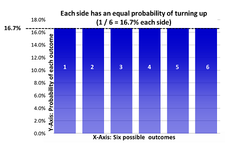
For example, consider rolling a six-sided die. Each outcome from 1 to 6 has a probability of 1/6. The probability distribution describes this pattern of probabilities across the possible outcomes.
Probability distributions are widely used in various disciplines such as mathematics, statistics, economics, engineering, finance, physics, biology, and data science. They allow researchers to analyze random phenomena, predict outcomes, and understand patterns in data.
Understanding probability distributions is essential for studying statistical inference, hypothesis testing, machine learning models, and stochastic processes. Many statistical methods rely on specific probability distributions to describe the behavior of data.
Probability distributions help answer important questions such as:
- What values can a random variable take?
- How likely is each value?
- How are probabilities distributed across outcomes?
By studying probability distributions, statisticians gain insight into the behavior of random variables and the structure of uncertain systems.
Random Variables and Probability Distributions


A probability distribution is closely related to the concept of a random variable.
A random variable is a variable whose value depends on the outcome of a random experiment. Instead of describing outcomes verbally, random variables represent outcomes numerically.
For example, when tossing two coins, the sample space is:
S = {HH, HT, TH, TT}
If we define a random variable X as the number of heads obtained, then:
X(HH) = 2
X(HT) = 1
X(TH) = 1
X(TT) = 0
Thus, the random variable X takes values:
0, 1, 2
The probability distribution of X describes the probability associated with each of these values.
The distribution might be represented as:
P(X = 0) = 1/4
P(X = 1) = 1/2
P(X = 2) = 1/4
This table represents the probability distribution of the random variable.
Probability distributions provide a complete description of the behavior of random variables.
Types of Probability Distributions

Probability distributions are broadly classified into two main types.
Discrete Probability Distributions
A discrete probability distribution describes random variables that take countable values.
Examples include:
- number of heads in coin tosses
- number of customers arriving at a store
- number of defective products in a batch
Discrete distributions are represented using a probability mass function (PMF).
Properties of PMF:
- P(X = x) ≥ 0 for all values of x
- Σ P(X = x) = 1
Examples of discrete distributions include binomial distribution, Poisson distribution, and geometric distribution.
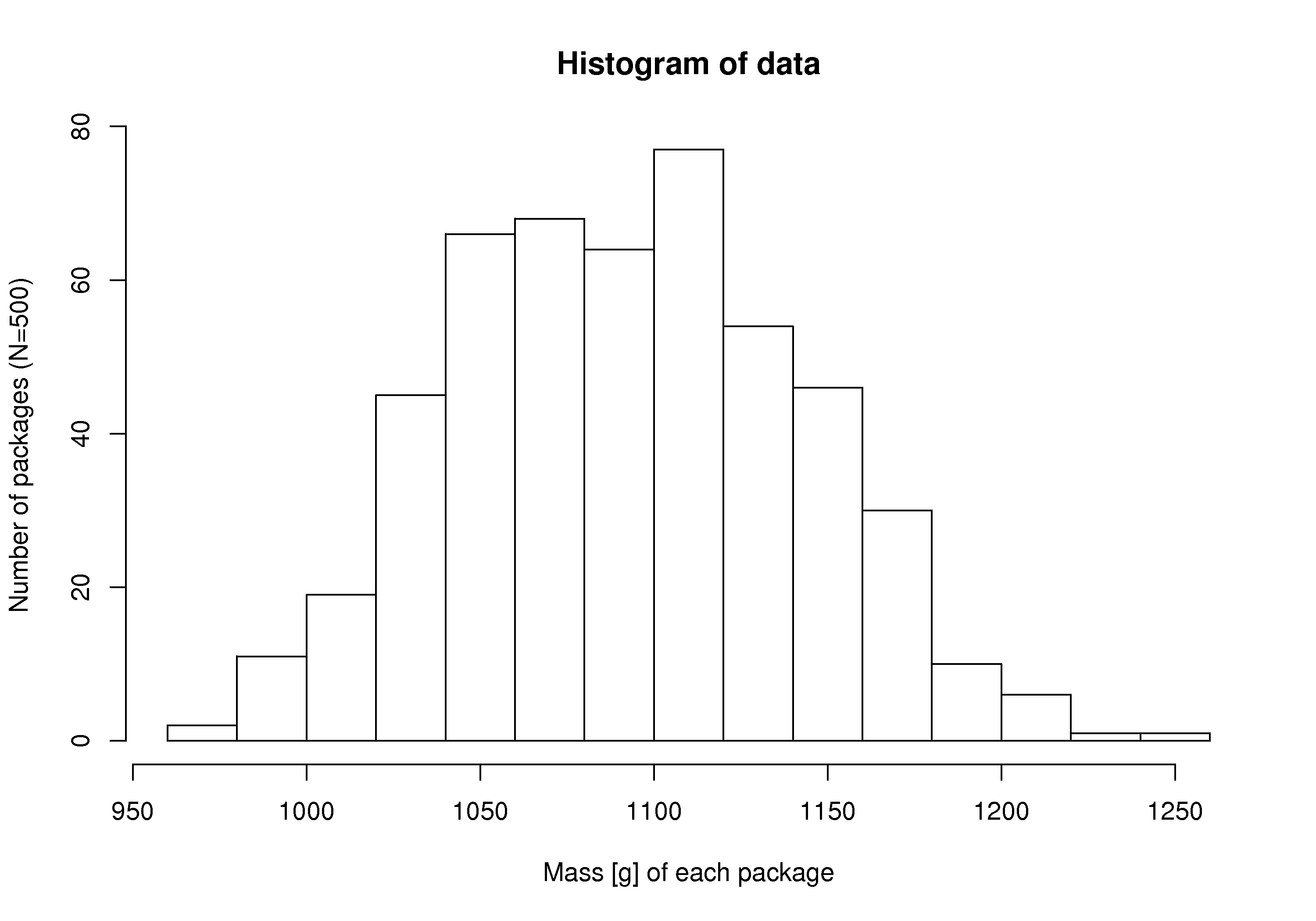
Continuous Probability Distributions
Continuous probability distributions describe variables that can take infinitely many values within a range.
Examples include:
- height of individuals
- temperature
- time required to complete a task
- weight of objects
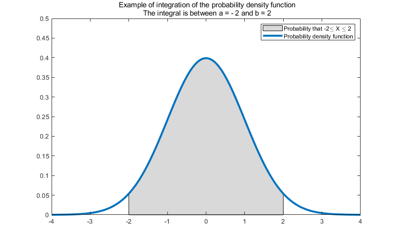
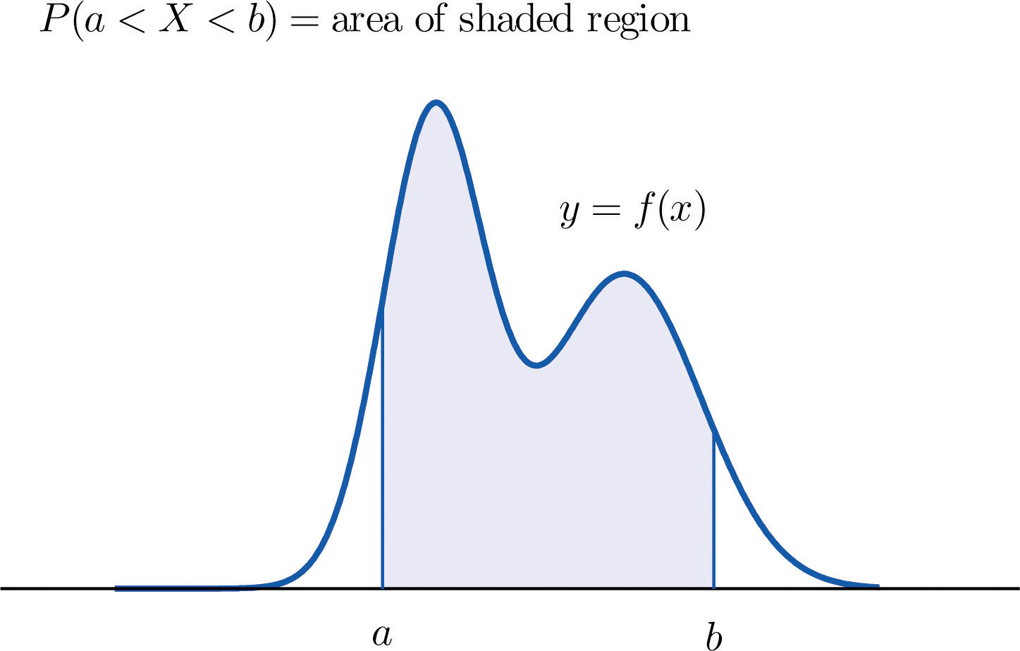
Continuous distributions are represented using a probability density function (PDF).
The probability of a value is determined by the area under the curve.
Total area under the probability density curve equals 1.
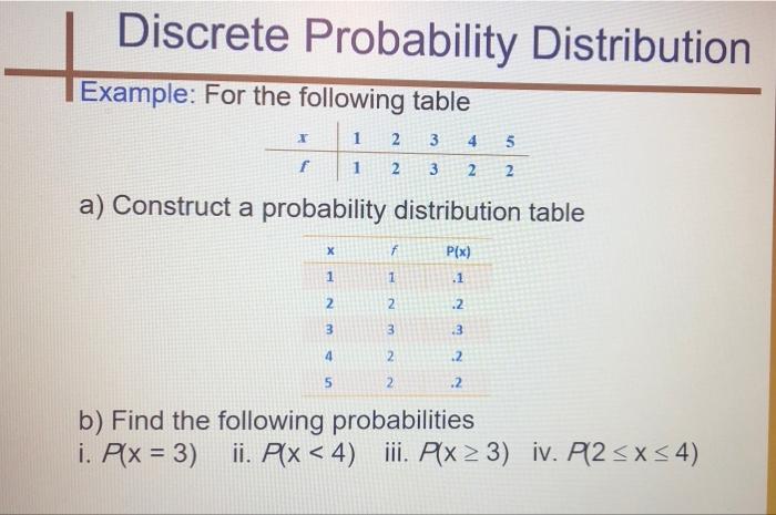
Probability Mass Function
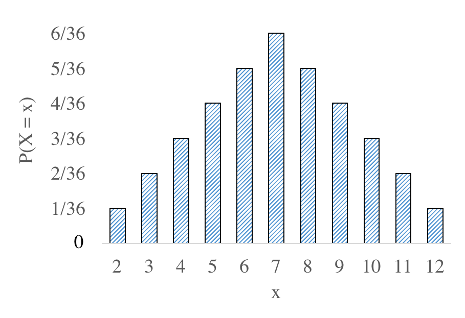


The probability mass function describes the probability distribution of a discrete random variable.
If X is a discrete random variable, the PMF is defined as:
P(X = x)
This function assigns probabilities to each possible value of X.
Example:
Suppose a die is rolled.
X = number obtained
The PMF is:
P(X = 1) = 1/6
P(X = 2) = 1/6
P(X = 3) = 1/6
P(X = 4) = 1/6
P(X = 5) = 1/6
P(X = 6) = 1/6
PMF graphs are usually represented using bar charts.
Probability Density Function
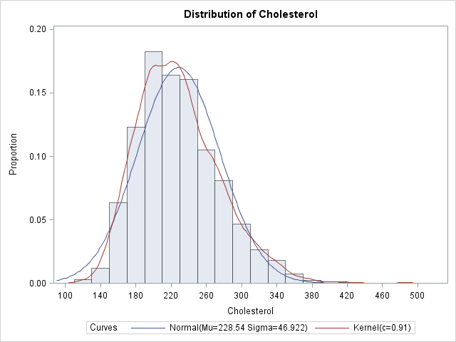
The probability density function describes the distribution of continuous random variables.
Unlike discrete distributions, the probability at a specific point is zero. Instead, probabilities are calculated over intervals.
Example:
P(a ≤ X ≤ b) = area under the curve between a and b
The PDF must satisfy the following properties:
- f(x) ≥ 0 for all x
- Total area under the curve = 1
Many well-known continuous distributions use probability density functions.
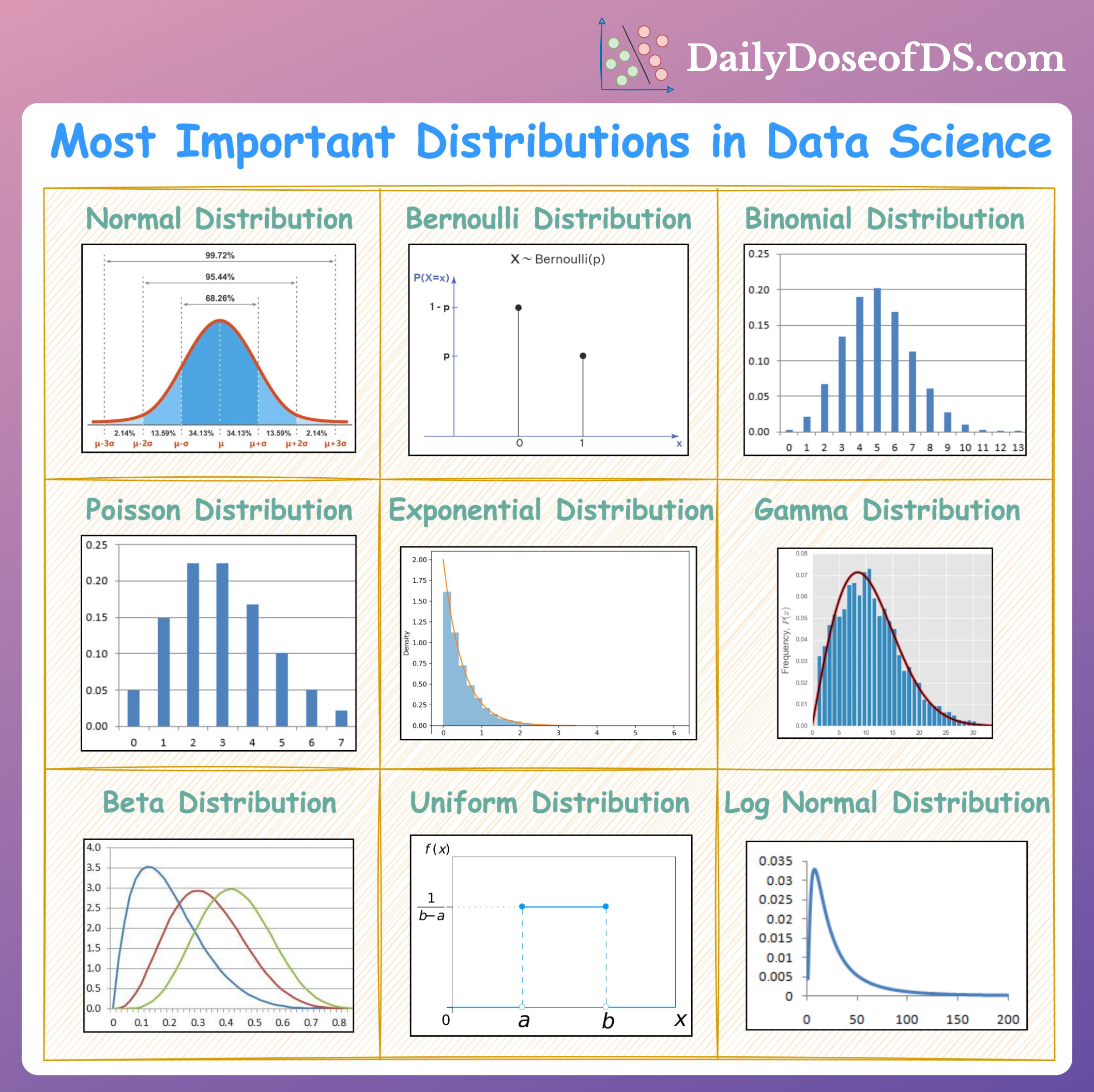
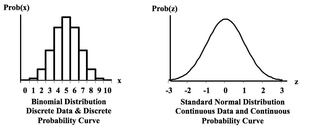
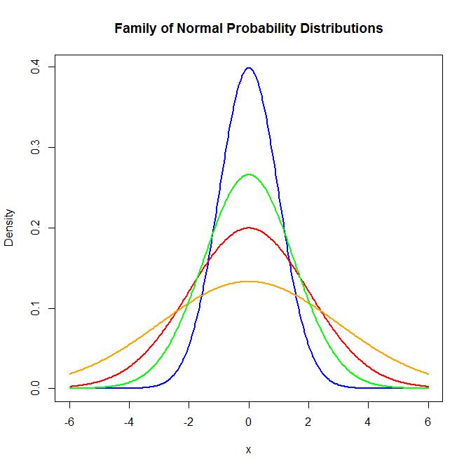
Normal Distribution


The normal distribution is one of the most important probability distributions in statistics.
It is also known as the Gaussian distribution.
Characteristics of the normal distribution:
- bell-shaped curve
- symmetric around the mean
- mean, median, and mode are equal
The probability density function is:
f(x) = (1 / (σ√2π)) e^(-(x − μ)² / (2σ²))
Where:
μ = mean
σ = standard deviation
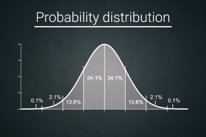
The empirical rule describes how data is distributed:
- 68% of data lies within 1 standard deviation
- 95% within 2 standard deviations
- 99.7% within 3 standard deviations
The normal distribution is widely used in natural sciences and social sciences.
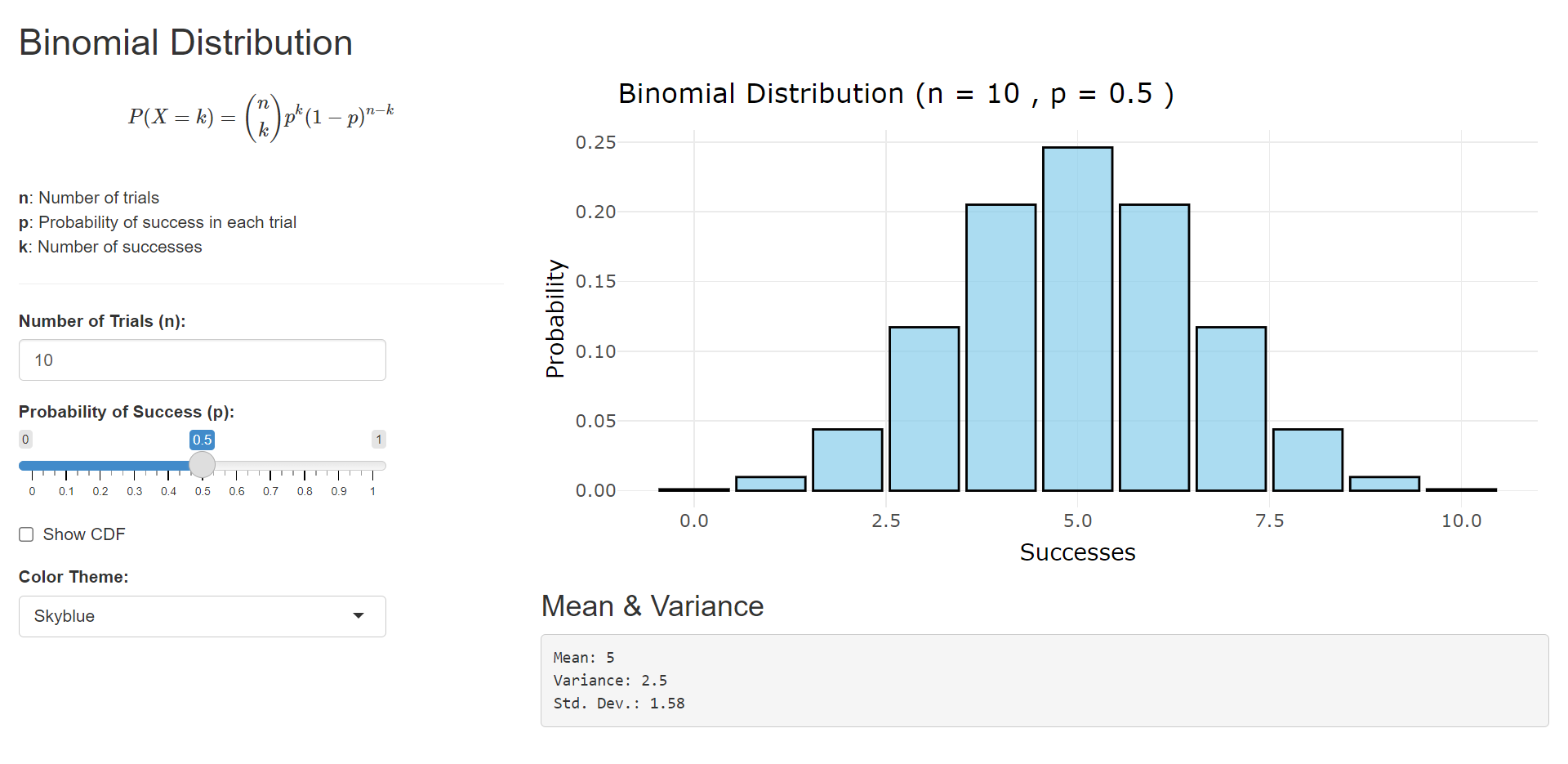
Binomial Distribution
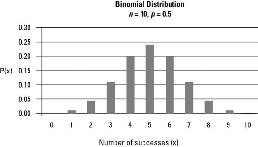
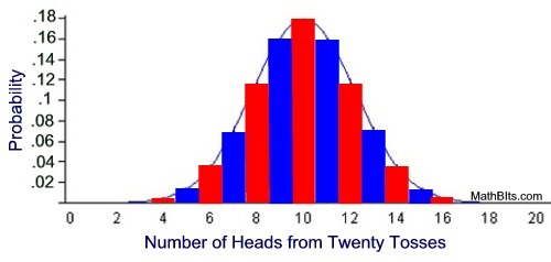


The binomial distribution describes the number of successes in a fixed number of independent trials.
Conditions for binomial distribution:
- Fixed number of trials
- Each trial has two outcomes
- Constant probability of success
The probability formula is:
P(X = k) = (nCk) p^k (1 − p)^(n − k)
Where:
n = number of trials
k = number of successes
p = probability of success
Example:
Number of heads obtained when tossing a coin multiple times.
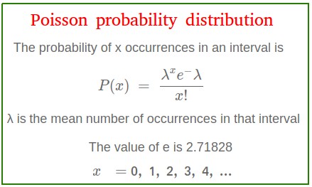
Poisson Distribution

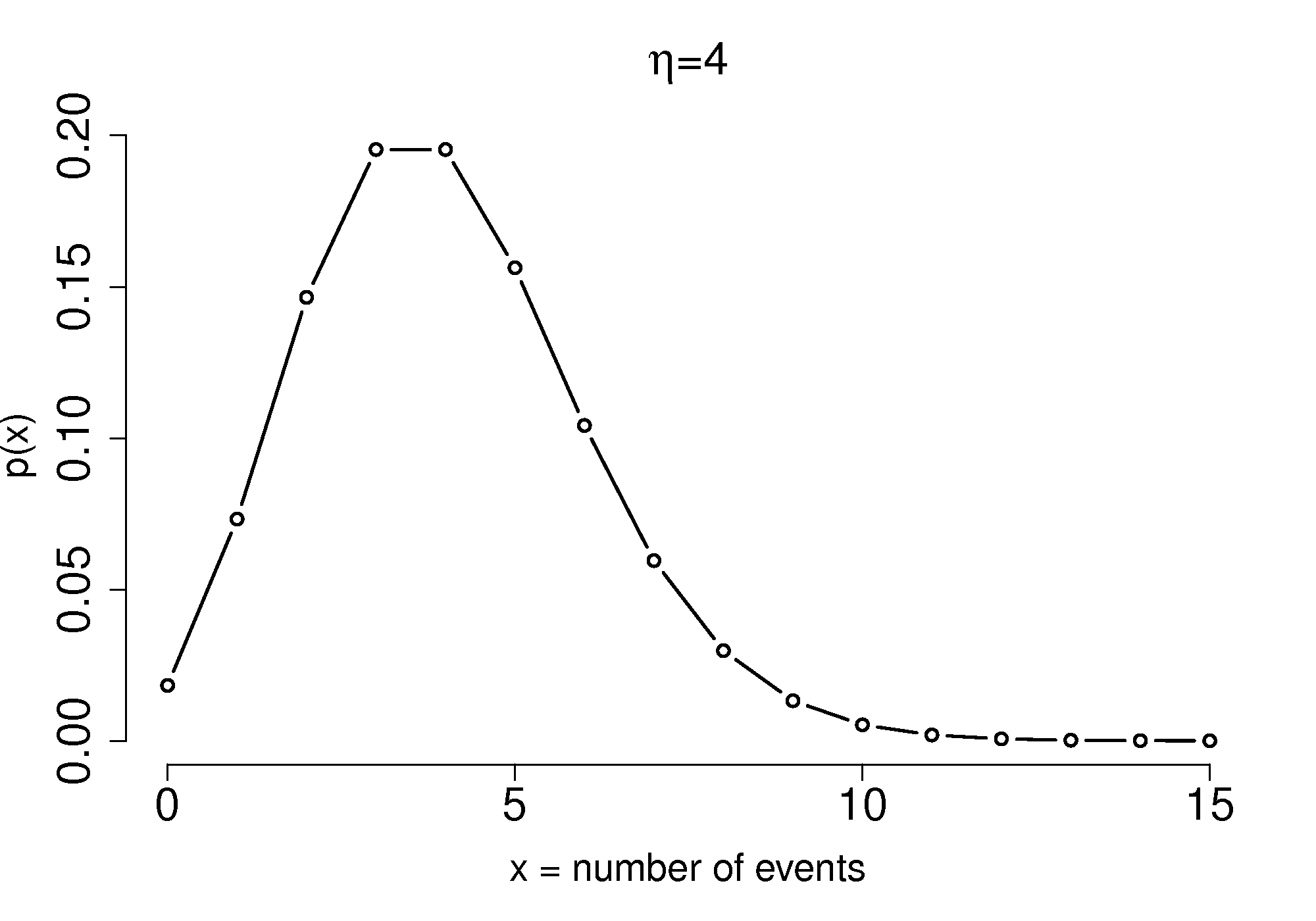
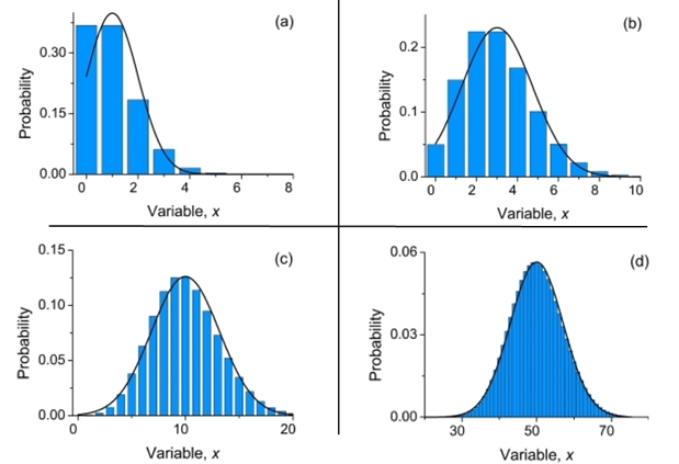

The Poisson distribution describes the probability of a certain number of events occurring in a fixed interval of time or space.
Examples include:
- number of phone calls received in an hour
- number of accidents on a road
- number of defects in manufactured items
The formula is:
P(X = k) = (λ^k e^−λ) / k!
Where:
λ represents the average rate of occurrence.
Poisson distribution is commonly used for modeling rare events.
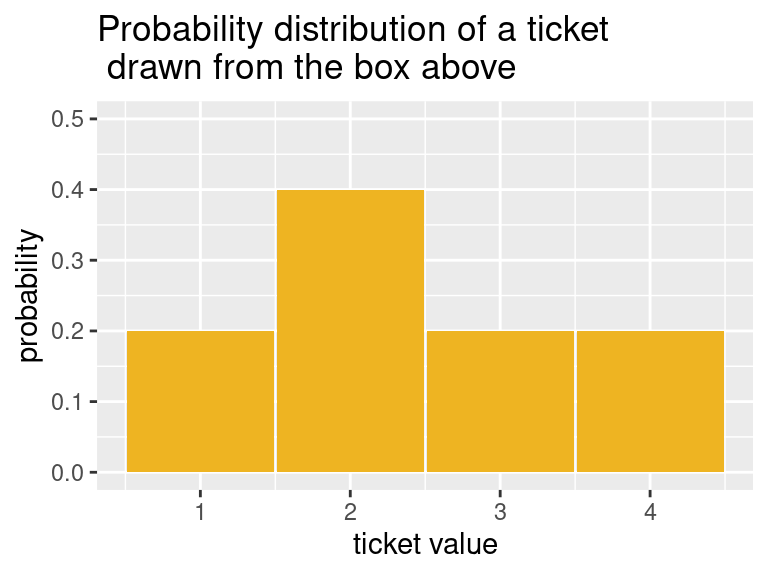
Uniform Distribution
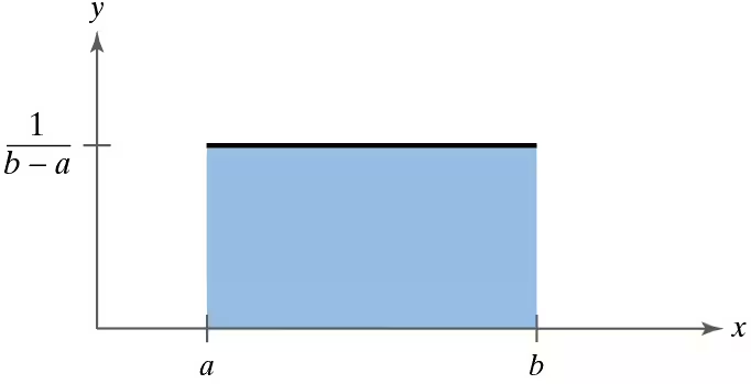


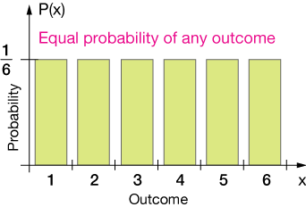
The uniform distribution occurs when all outcomes have equal probability.
Example:
Rolling a fair die.
Each outcome has probability:
1/6
In continuous uniform distribution, the probability density remains constant across an interval.
Uniform distributions are used in computer simulations and random number generation.
Applications of Probability Distributions

Probability distributions are widely used in many real-world applications.
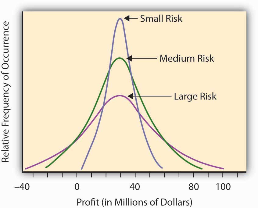
Finance
Used to model stock market behavior and financial risks.
Engineering
Used in reliability analysis and quality control.
Medicine
Used to analyze medical test results and disease spread.
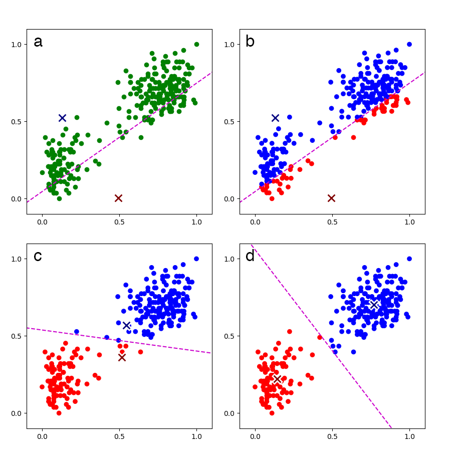
Data Science
Machine learning algorithms rely heavily on probability distributions.
Weather Forecasting
Meteorologists use probability distributions to predict weather conditions.
These applications highlight the importance of probability distributions in modern analysis.
Importance of Probability Distributions
Probability distributions play a critical role in statistical modeling and decision-making under uncertainty.
They help researchers:
- describe random variables mathematically
- analyze patterns in data
- estimate probabilities of events
- develop predictive models
Many statistical techniques rely on probability distributions to make accurate predictions and conclusions.
Understanding probability distributions provides a foundation for advanced statistical learning.
Conclusion
Probability distributions are essential tools in probability theory and statistics. They describe how probabilities are assigned to values of random variables and help analyze uncertain events.
There are two main types of probability distributions: discrete and continuous. Important distributions include the binomial distribution, Poisson distribution, uniform distribution, and normal distribution.
These distributions are widely used in fields such as mathematics, economics, engineering, finance, and data science. By studying probability distributions, researchers can better understand patterns in data and make informed decisions under uncertainty.