Tag Archives: statistics probability learning material

Basic Probability Rules in Mathematics

Image
Image
Image
Image

Introduction to Probability

Probability is a branch of mathematics that deals with uncertainty and the likelihood of events occurring. It provides a numerical measure that describes how likely an event is to happen in a random experiment. Probability plays an essential role in statistics, decision making, risk assessment, scientific research, and many real-world applications.

In everyday life, people encounter uncertainty frequently. For example, predicting weather conditions, determining the chance of winning a game, or estimating the likelihood of a disease occurring are all situations involving probability. Mathematical probability allows us to analyze such situations logically and quantitatively.

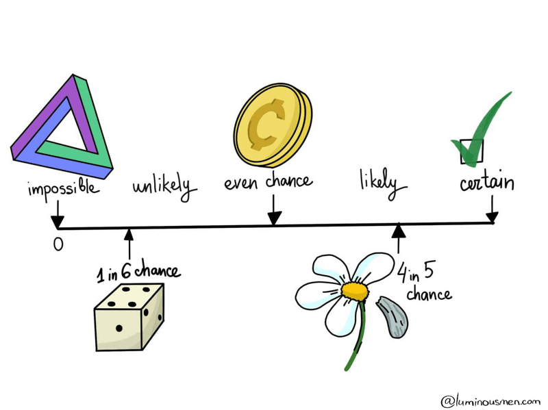
Probability values range between 0 and 1, where:

  • 0 represents an impossible event
  • 1 represents a certain event

Any event whose probability lies between these values indicates varying levels of likelihood.

The study of probability began in the seventeenth century when mathematicians started analyzing games of chance. Today, probability theory has become an essential component of mathematics, statistics, economics, engineering, and computer science.

Understanding basic probability rules helps students analyze random events, interpret data, and make predictions about uncertain outcomes.


Random Experiments and Sample Space

Image
Image
Image
Image

Random Experiment

A random experiment is an experiment or process whose outcome cannot be predicted with certainty.

Examples include:

  • tossing a coin
  • rolling a die
  • drawing a card from a deck
  • measuring rainfall in a city

Even though the exact outcome is unknown, the possible outcomes are known.
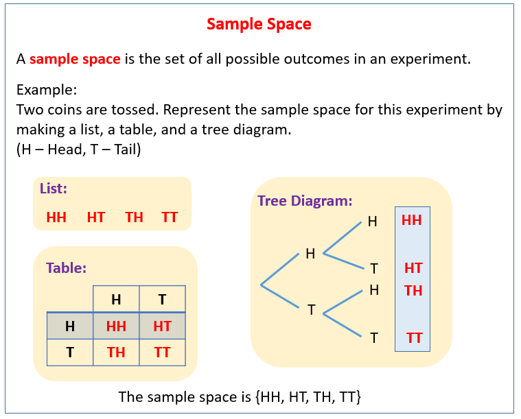
Sample Space

The sample space is the set of all possible outcomes of a random experiment.

Example:

When tossing a coin:

S = {H, T}

Where:

H = Head
T = Tail

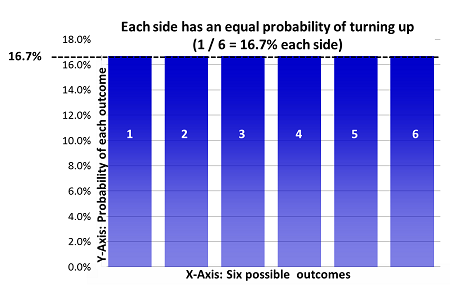
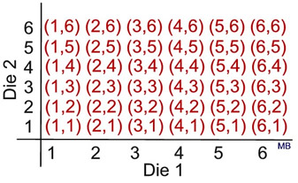
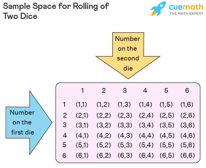
When rolling a six-sided die:

S = {1, 2, 3, 4, 5, 6}

The sample space forms the basis for calculating probabilities.

Event

An event is a subset of the sample space.

Example:

Event A: Getting an even number when rolling a die.

A = {2, 4, 6}

Events are the outcomes we are interested in analyzing.


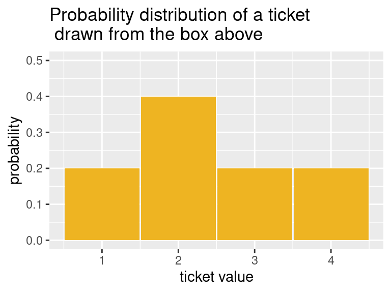
Classical Definition of Probability

Image
Image
Image
Image

The classical definition of probability is based on equally likely outcomes.

If an event A occurs in m ways out of n possible outcomes, the probability of event A is:

P(A) = m / n

Where:

  • m = number of favorable outcomes
  • n = total number of possible outcomes

Example:

Consider rolling a die.

Probability of getting a 3:

P(3) = 1 / 6

Probability of getting an even number:

Even numbers = {2, 4, 6}

P(Even) = 3 / 6 = 1 / 2

This formula is used when outcomes are equally likely.


Basic Probability Rules

Image
Image
Image
Image

Probability theory is governed by several fundamental rules that help calculate probabilities for different types of events.

These rules form the foundation of probability calculations.

The main probability rules include:

  • Range rule
  • Complement rule
  • Addition rule
  • Multiplication rule
  • Conditional probability rule

Each rule helps solve different types of probability problems.


Rule 1: Range Rule of Probability

The probability of any event must lie between 0 and 1.

Mathematically:

0 ≤ P(A) ≤ 1

Examples:

Impossible event:

P(A) = 0

Certain event:

P(A) = 1

Example:

Probability that the sun rises tomorrow ≈ 1.

Probability of drawing a red ball from a bag with only blue balls = 0.

This rule ensures probabilities remain within valid limits.


Rule 2: Complement Rule

Image
Image
Image
Image

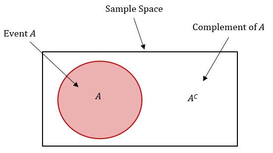
The complement of an event represents outcomes where the event does not occur.

If event A occurs with probability P(A), then its complement is denoted by A’.

Complement rule:

P(A’) = 1 − P(A)

Example:

Probability of getting a head when tossing a coin:

P(H) = 1/2

Probability of not getting a head:

P(H’) = 1 − 1/2 = 1/2

Another example:

If the probability of rain tomorrow is 0.3, the probability that it will not rain is:

0.7

Complement rule simplifies probability calculations.


Rule 3: Addition Rule of Probability

Image
Image
Image
Image

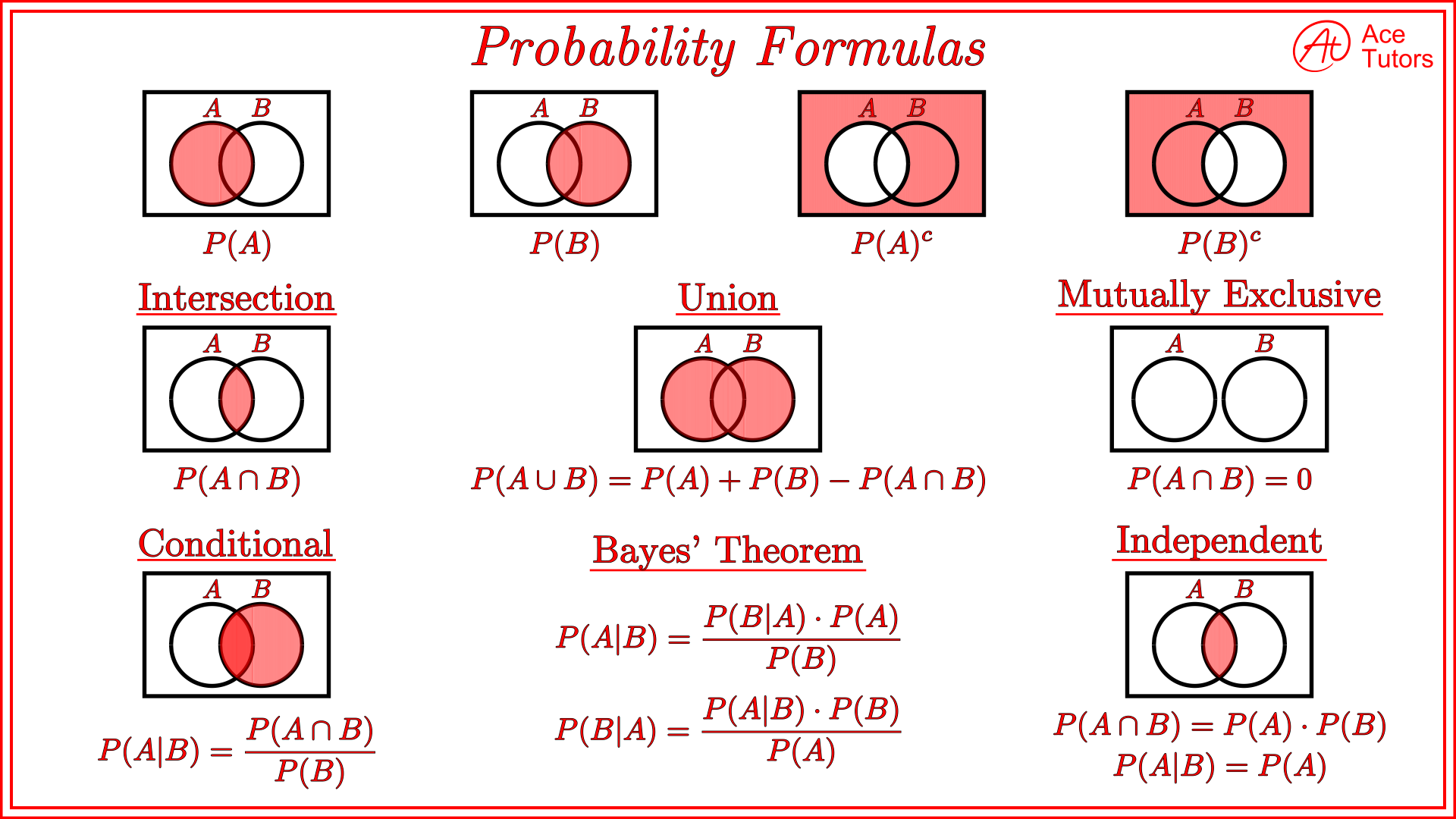
The addition rule is used to calculate the probability that at least one of two events occurs.

For Mutually Exclusive Events

If events A and B cannot occur simultaneously:

P(A ∪ B) = P(A) + P(B)

Example:

Rolling a die.

Event A: Getting 1
Event B: Getting 2

P(A ∪ B) = 1/6 + 1/6 = 1/3

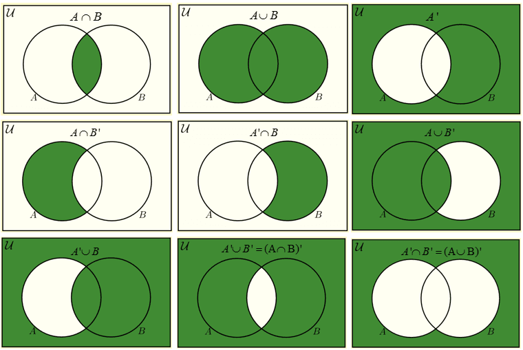
For Non-Mutually Exclusive Events

If events overlap:

P(A ∪ B) = P(A) + P(B) − P(A ∩ B)

Where:

A ∩ B represents the intersection of events.

This rule avoids double-counting shared outcomes.


Rule 4: Multiplication Rule of Probability

Image
Image
Image
Image

The multiplication rule calculates the probability that two events occur together.

Independent Events

Events are independent if the occurrence of one does not affect the other.

Formula:

P(A ∩ B) = P(A) × P(B)
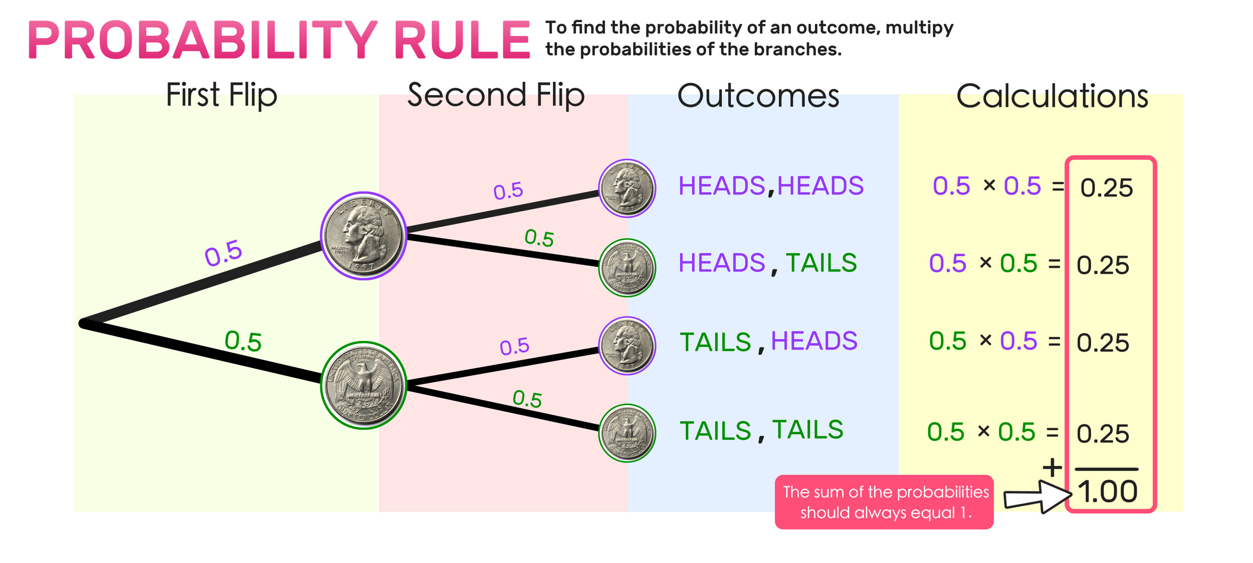
Example:

Tossing two coins.

Probability of two heads:

P(HH) = 1/2 × 1/2 = 1/4

Dependent Events

Events are dependent if one event affects the probability of the other.

Formula:

P(A ∩ B) = P(A) × P(B|A)

Where:

P(B|A) = probability of B given that A occurred.


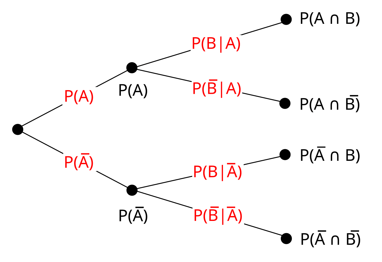
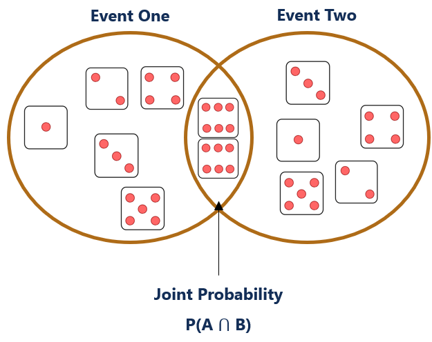
Conditional Probability

Image
Image
Image
Image

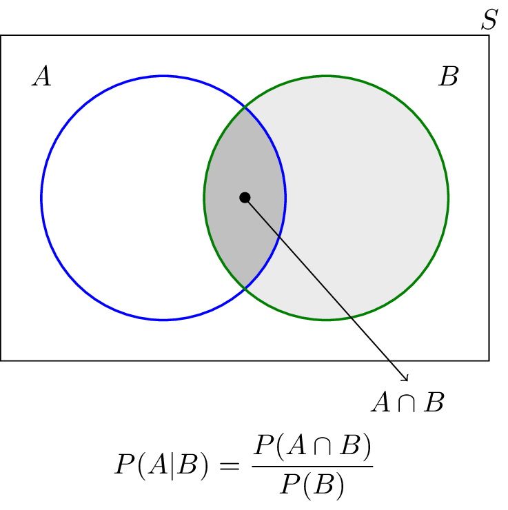
Conditional probability measures the probability of an event given that another event has already occurred.

Formula:

P(A|B) = P(A ∩ B) / P(B)

Example:

Suppose a card is drawn from a deck.

Event A: Card is a king
Event B: Card is a face card

P(A|B) = number of kings / number of face cards

= 4 / 12 = 1/3

Conditional probability is widely used in statistics, machine learning, and decision-making.


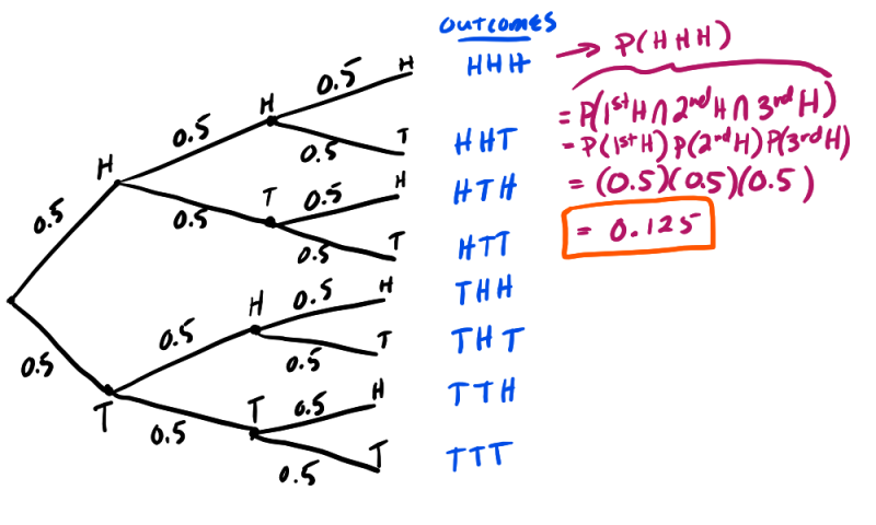
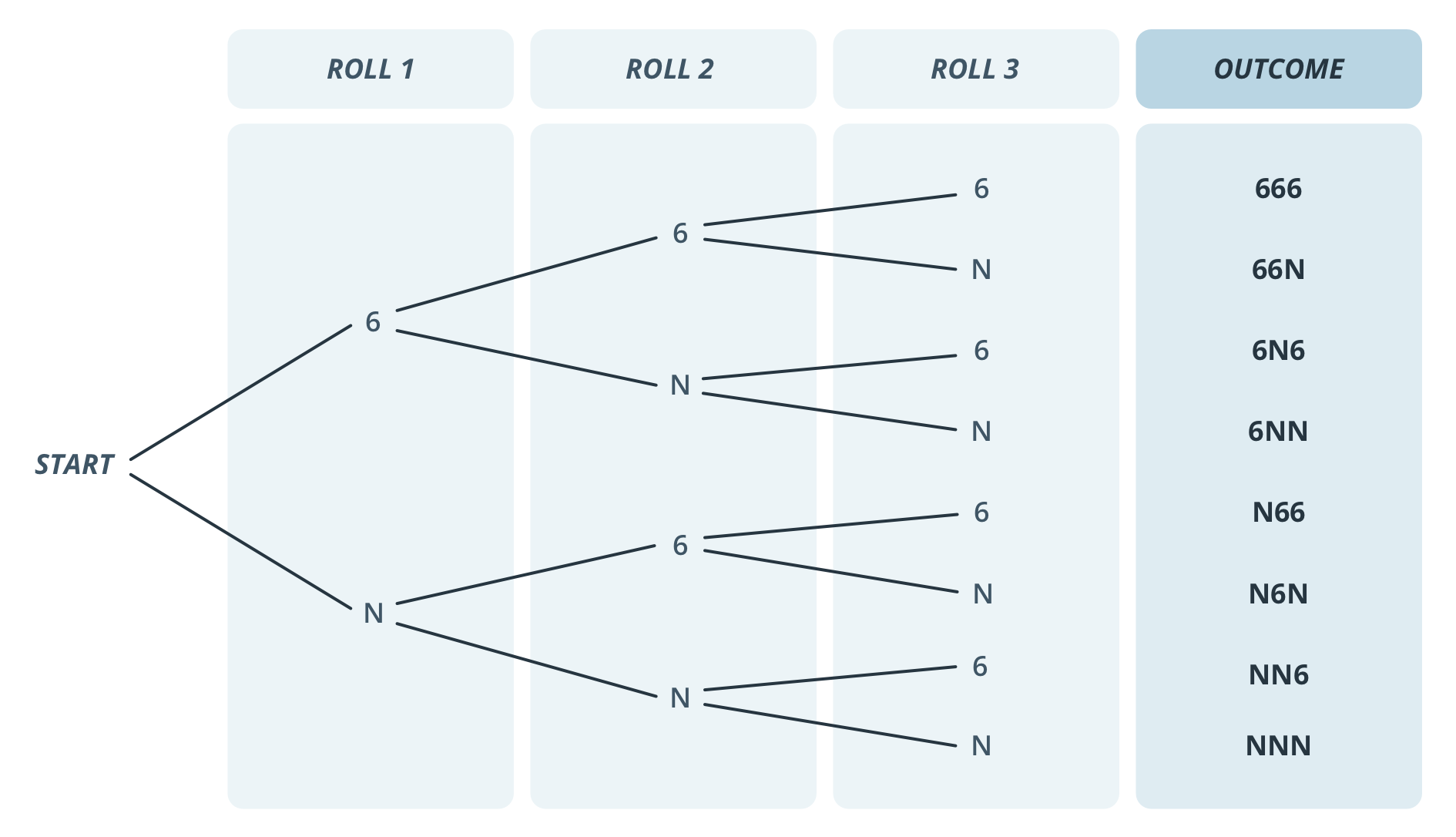
Probability Using Tree Diagrams

Image
Image
Image
Image

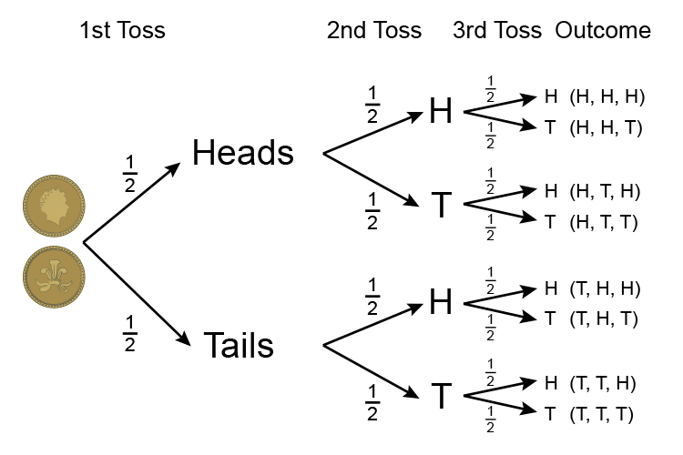
Tree diagrams provide a visual way to analyze probability experiments involving multiple stages.

Each branch represents a possible outcome.

Example:

Two coin tosses produce the outcomes:

HH, HT, TH, TT

Each outcome has probability:

1/4

Tree diagrams make probability calculations easier to understand.


Applications of Basic Probability Rules

Image
Image
Image
Image

Basic probability rules are used in many practical applications.

Weather Forecasting

Meteorologists use probability to predict weather conditions.

Insurance

Insurance companies estimate risks using probability.

Medical Diagnosis

Doctors use probability models to assess disease likelihood.

Finance

Investors analyze risk and return using probability theory.

Artificial Intelligence

Machine learning algorithms rely on probability models.

These applications demonstrate the importance of probability in decision-making.


Importance of Basic Probability Rules

Basic probability rules provide a framework for analyzing uncertain events.

They help:

  • calculate likelihood of outcomes
  • analyze random experiments
  • develop statistical models
  • support decision making under uncertainty

Understanding these rules forms the foundation for advanced topics in probability theory and statistics.


Conclusion

Basic probability rules are essential principles used to analyze random events and calculate the likelihood of outcomes. These rules include the complement rule, addition rule, multiplication rule, and conditional probability rule.

By applying these rules, mathematicians and statisticians can solve complex probability problems and interpret uncertain situations effectively.

Probability theory plays a critical role in many fields including science, economics, engineering, data science, and artificial intelligence. Mastering the basic rules of probability helps students develop logical thinking and analytical skills needed for advanced statistical analysis.

Understanding probability not only improves mathematical knowledge but also helps individuals make better decisions in everyday life.


Tags

Probability Distributions in Mathematics and Statistics

Image
Image
Image
Image

Introduction to Probability Distributions

Probability distributions are fundamental concepts in probability theory and statistics that describe how the values of a random variable are distributed. In simple terms, a probability distribution provides a mathematical description of the likelihood of different outcomes in an experiment or random process.

In many real-world situations, outcomes are uncertain. For example, when tossing a coin, rolling a die, or measuring rainfall in a city, the exact result cannot always be predicted with certainty. However, probability distributions allow us to understand the pattern of possible outcomes and assign probabilities to them.

A probability distribution tells us:

  • What values a random variable can take
  • How likely each value is to occur

For instance, when rolling a fair six-sided die, the probability of each number from 1 to 6 occurring is equal. The probability distribution of the die shows that each outcome has a probability of 1/6.

Probability distributions are widely used in many fields including mathematics, statistics, economics, engineering, physics, finance, biology, and machine learning. They help researchers model uncertainty, analyze data, and make predictions about future events.

Understanding probability distributions is essential for advanced statistical analysis, hypothesis testing, and decision-making under uncertainty.


Random Variables

Image
Image
Image
Image

Before studying probability distributions, it is important to understand the concept of random variables.

A random variable is a variable whose value is determined by the outcome of a random experiment.

For example:

  • The number obtained when rolling a die
  • The number of customers entering a store in an hour
  • The amount of rainfall in a day
  • The height of individuals in a population

Random variables can take different numerical values depending on the outcome of the experiment.

There are two main types of random variables:

  1. Discrete Random Variables
  2. Continuous Random Variables

These types lead to two major categories of probability distributions.


Discrete Probability Distributions

Image
Image
Image
Image

A discrete probability distribution describes probabilities for random variables that take countable values.

Examples of discrete random variables include:

  • number of heads in coin tosses
  • number of defective products in a batch
  • number of students in a classroom

Discrete probability distributions use a probability mass function (PMF).

The PMF gives the probability that a random variable equals a particular value.

Example:

Suppose a fair coin is tossed twice. Possible outcomes are:

HH, HT, TH, TT

Let X represent the number of heads.

Possible values:

0, 1, 2

The probability distribution is:

P(X = 0) = 1/4
P(X = 1) = 2/4
P(X = 2) = 1/4

This table represents the probability distribution.

The probabilities must satisfy two conditions:

  1. Each probability is between 0 and 1.
  2. The sum of probabilities equals 1.

Discrete probability distributions are often represented using bar charts.


Continuous Probability Distributions

Image
Image
Image
Image

Continuous probability distributions describe random variables that can take infinitely many values within a given range.

Examples include:

  • height of people
  • temperature
  • time required to complete a task
  • weight of objects

Unlike discrete distributions, continuous distributions use a probability density function (PDF).

The probability of a value is determined by the area under the curve.

For continuous distributions:

P(a ≤ X ≤ b) = area under the curve between a and b.

The total area under the curve equals 1.

Continuous probability distributions are represented using smooth curves rather than bars.


Normal Distribution

Image
Image
Image
Image

The normal distribution is one of the most important probability distributions in statistics.

It is also called the Gaussian distribution.

The normal distribution has the following characteristics:

  • symmetric bell-shaped curve
  • mean, median, and mode are equal
  • data is concentrated around the mean

The probability density function of the normal distribution is:

f(x) = (1 / (σ√2π)) e^(-(x−μ)² / 2σ²)

Where:

μ = mean
σ = standard deviation

One important property of the normal distribution is the empirical rule.

According to this rule:

  • 68% of data lies within 1 standard deviation of the mean
  • 95% lies within 2 standard deviations
  • 99.7% lies within 3 standard deviations

Normal distribution appears in many natural phenomena such as heights, exam scores, and measurement errors.


Binomial Distribution

Image
Image
Image
Image

The binomial distribution is a discrete probability distribution that describes the number of successes in a fixed number of independent trials.

Conditions for binomial distribution:

  1. Fixed number of trials
  2. Each trial has two outcomes (success or failure)
  3. Probability of success is constant

The probability formula is:

P(X = k) = (nCk) p^k (1 − p)^(n − k)

Where:

n = number of trials
k = number of successes
p = probability of success

Example:

If a coin is tossed 5 times, the binomial distribution can determine the probability of obtaining exactly 3 heads.


Poisson Distribution

Image
Image
Image
Image

The Poisson distribution models the number of events occurring in a fixed interval of time or space.

Examples include:

  • number of phone calls received in an hour
  • number of accidents on a road
  • number of typing errors on a page

The formula for Poisson distribution is:

P(X = k) = (λ^k e^−λ) / k!

Where:

λ = average number of events
k = number of occurrences

The Poisson distribution is commonly used for modeling rare events.


Uniform Distribution

Image
Image
Image
Image

The uniform distribution occurs when all outcomes are equally likely.

Example:

Rolling a fair die.

Each number from 1 to 6 has equal probability.

In continuous uniform distribution, the probability density is constant across the interval.

Uniform distributions are used in simulations and computer algorithms.


Exponential Distribution

Image
Image
Image
Image

The exponential distribution models the time between events in a Poisson process.

Examples include:

  • time between arrivals of customers
  • time until a machine fails
  • waiting time for a bus

The probability density function is:

f(x) = λ e^(-λx)

Where λ is the rate parameter.

This distribution is widely used in reliability analysis and queueing theory.


Applications of Probability Distributions

Image
Image
Image
Image

Probability distributions are used in many practical applications.

Finance

Used to model stock market returns and financial risk.

Engineering

Used in reliability analysis and quality control.

Medicine

Used to analyze clinical trials and disease spread.

Data Science

Machine learning algorithms rely on probability distributions.

Economics

Used to study income distribution and market behavior.

These applications highlight the importance of probability distributions.


Importance of Probability Distributions

Probability distributions play a central role in statistics and probability theory.

They help:

  • model uncertainty
  • analyze random phenomena
  • make predictions
  • support statistical inference

Many advanced statistical methods depend on probability distributions.

Understanding them allows researchers to interpret data more effectively.


Conclusion

Probability distributions provide mathematical models that describe how random variables behave. They help assign probabilities to possible outcomes and explain how data values are distributed.

There are two main categories of probability distributions: discrete and continuous. Important distributions include binomial, Poisson, normal, uniform, and exponential distributions.

These distributions are essential tools in mathematics, statistics, science, engineering, economics, and data analysis. By understanding probability distributions, researchers can analyze uncertainty, model real-world phenomena, and make informed decisions.

Probability distributions form the foundation of modern statistics and are crucial for studying randomness and variability in data.


Tags