Tag Archives: systems of linear equations

Matrices

Image
Image
Image
Image

1. Introduction to Matrices

A matrix is a rectangular arrangement of numbers, symbols, or expressions organized in rows and columns. Matrices are one of the most important structures in mathematics and play a crucial role in algebra, engineering, physics, statistics, computer science, economics, and data science.

Matrices are particularly useful when dealing with large sets of numbers, solving systems of linear equations, performing transformations in geometry, and modeling real-world problems.

The plural of matrix is matrices.

Matrices were first introduced in the 19th century by mathematicians such as Arthur Cayley, who developed matrix algebra. Since then, matrices have become a fundamental component of linear algebra, which is widely used in scientific and technological applications.

For example, consider a simple table representing students’ marks:

MathScienceEnglish
857890
888291

This table can be represented as a matrix:

A =
[ 85 78 90 ]
[ 88 82 91 ]

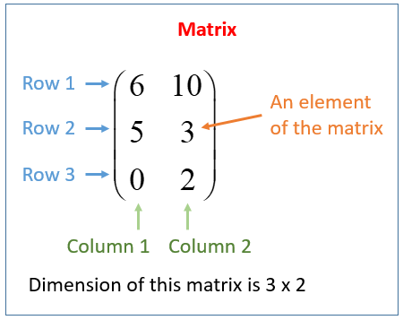
Each number in a matrix is called an element or entry.


2. Structure of a Matrix

A matrix is defined by:

  • Rows
  • Columns

If a matrix has m rows and n columns, it is called an m × n matrix.

Example:

A =
[ 1 2 3 ]
[ 4 5 6 ]

This matrix has:

Rows = 2
Columns = 3

So it is called a 2 × 3 matrix.


General Form of a Matrix

A matrix is usually written as:

A = [aᵢⱼ]

Where:

  • i represents row number
  • j represents column number

Example:

A =
[ a11 a12 a13 ]
[ a21 a22 a23 ]

Here:

a21 means element in 2nd row and 1st column.


3. Representation of Matrices

Matrices are represented using capital letters.

Examples:

A, B, C, M, X

Example matrix:

A =
[ 2 5 ]
[ 3 7 ]

The elements are:

a11 = 2
a12 = 5
a21 = 3
a22 = 7


4. Order of a Matrix

The order of a matrix describes its size.

Order = rows × columns

Examples:

MatrixOrder
[1 2]1 × 2
[3 4; 5 6]2 × 2
[1 2 3; 4 5 6; 7 8 9]3 × 3

5. Types of Matrices

Matrices can be classified into several types based on their structure.


Row Matrix

A matrix with only one row.

Example:

A = [ 2 4 6 8 ]

Order:

1 × 4


Column Matrix

A matrix with only one column.

Example:

A =
[3]
[5]
[7]

Order:

3 × 1


Rectangular Matrix

If rows ≠ columns.

Example:

2 × 3 matrix

A =
[1 2 3]
[4 5 6]


Square Matrix

A matrix with equal rows and columns.

Example:

A =
[1 2]
[3 4]

Order:

2 × 2

Square matrices are very important because many operations like determinants and inverses are defined for them.


Zero Matrix

A matrix whose elements are all zero.

Example:

A =
[0 0]
[0 0]


Diagonal Matrix

A square matrix where all elements except the diagonal are zero.

Example:

A =
[5 0 0]
[0 3 0]
[0 0 7]


Identity Matrix

A square matrix where diagonal elements are 1 and others are 0.

Example:

I =
[1 0 0]
[0 1 0]
[0 0 1]

Identity matrix behaves like number 1 in multiplication.


Scalar Matrix

A diagonal matrix with equal diagonal elements.

Example:

A =
[4 0 0]
[0 4 0]
[0 0 4]


Upper Triangular Matrix

Elements below the diagonal are zero.

Example:

A =
[2 4 6]
[0 5 7]
[0 0 9]


Lower Triangular Matrix

Elements above the diagonal are zero.

Example:

A =
[3 0 0]
[5 6 0]
[7 8 9]


6. Equality of Matrices

Two matrices are equal if:

  1. Their orders are equal
  2. Corresponding elements are equal

Example:

A =
[1 2]
[3 4]

B =
[1 2]
[3 4]

Therefore:

A = B


7. Addition of Matrices

Matrices can be added if they have the same order.

Example:

A =
[1 2]
[3 4]

B =
[5 6]
[7 8]

A + B =

[1+5 2+6]
[3+7 4+8]

Result:

[6 8]
[10 12]


Properties of Matrix Addition

  1. Commutative Property

A + B = B + A

  1. Associative Property

(A + B) + C = A + (B + C)

  1. Additive Identity

A + 0 = A

  1. Additive Inverse

A + (-A) = 0


8. Subtraction of Matrices

Matrix subtraction is defined as:

A − B = A + (−B)

Example:

A =
[8 6]
[4 2]

B =
[3 1]
[5 2]

A − B =

[5 5]
[-1 0]


9. Scalar Multiplication

Multiplying a matrix by a number.

Example:

A =
[2 4]
[6 8]

3A =

[6 12]
[18 24]


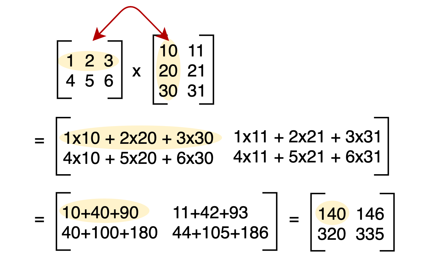
10. Matrix Multiplication

Matrix multiplication is different from ordinary multiplication.

Condition:

Columns of first matrix = rows of second matrix

If

A = m × n
B = n × p

Then:

AB = m × p


Example:

A =
[1 2]
[3 4]

B =
[5 6]
[7 8]

AB =

[1×5 + 2×7 1×6 + 2×8]
[3×5 + 4×7 3×6 + 4×8]

Result:

[19 22]
[43 50]


Properties of Matrix Multiplication

  1. Not commutative

AB ≠ BA

  1. Associative

(A B)C = A(B C)

  1. Distributive

A(B + C) = AB + AC


11. Transpose of a Matrix

The transpose of a matrix is obtained by interchanging rows and columns.

If A is matrix:

Aᵀ is transpose.

Example:

A =
[1 2 3]
[4 5 6]

Aᵀ =

[1 4]
[2 5]
[3 6]


12. Determinant of a Matrix

Determinants are defined only for square matrices.

For a 2×2 matrix

A =
[ a b ]
[ c d ]

Determinant:

|A| = ad − bc

Example:

| 2 3 |
| 4 5 |

= (2×5) − (3×4)
= 10 − 12
= −2


13. Inverse of a Matrix

A matrix inverse is similar to reciprocal.

If:

A⁻¹ exists then

A × A⁻¹ = I

Where I is identity matrix.

For 2×2 matrix:

A =
[ a b ]
[ c d ]

Inverse:

1/(ad − bc)

[ d −b ]
[ −c a ]


14. Rank of a Matrix

The rank of a matrix is the maximum number of independent rows or columns.

Rank tells:

  • how many independent equations exist
  • whether system has solution

15. Elementary Operations on Matrices

Three basic operations:

  1. Row swapping
  2. Row multiplication
  3. Row addition

Used in solving equations.


16. Systems of Linear Equations Using Matrices

Example system:

2x + y = 5
x + 3y = 7

Matrix form:

AX = B

A = coefficient matrix
X = variable matrix
B = constant matrix

Using inverse:

X = A⁻¹B


17. Applications of Matrices

Matrices are used in many fields.


Computer Graphics

Matrices perform transformations:

  • Rotation
  • Scaling
  • Translation

Used in video games and animation.


Physics

Matrices describe:

  • Quantum mechanics
  • Electromagnetism
  • Mechanics

Engineering

Used in:

  • Structural analysis
  • Electrical circuits
  • Robotics

Economics

Matrices help analyze:

  • Input-output models
  • Economic forecasting

Statistics

Matrices represent datasets and perform calculations like:

  • covariance
  • regression
  • machine learning algorithms

Cryptography

Matrices are used in encryption methods like the Hill cipher.


Artificial Intelligence

Matrices represent:

  • neural networks
  • machine learning data
  • deep learning models

18. Matrices in Computer Science

Matrices play a major role in:

  • Image processing
  • Data compression
  • Graph theory
  • Machine learning

Example:

Images are stored as pixel matrices.


19. Eigenvalues and Eigenvectors

For a matrix A:

Av = λv

Where:

λ = eigenvalue
v = eigenvector

These concepts are used in:

  • vibration analysis
  • facial recognition
  • Google PageRank

20. Importance of Matrices

Matrices simplify complex mathematical problems.

They help in:

  • solving simultaneous equations
  • modeling systems
  • handling large datasets
  • performing transformations

Matrices are essential tools in modern science and technology.


Conclusion

Matrices are powerful mathematical tools that organize numbers into structured arrays. They play a central role in linear algebra and are widely used in mathematics, engineering, physics, computer science, economics, and artificial intelligence. By representing complex data and relationships in a compact form, matrices make it easier to perform calculations, solve equations, and analyze systems.

Matrix operations such as addition, multiplication, transpose, determinants, and inverses allow mathematicians and scientists to model real-world problems effectively. Applications of matrices extend to computer graphics, machine learning, quantum physics, robotics, and cryptography.

Understanding matrices provides a foundation for advanced mathematical concepts and modern technological developments.


Tags

Linear Equations in Mathematics

Image
Image
Image
Image

Tags:


Linear Equations in Mathematics

Linear equations are one of the most fundamental topics in algebra and mathematics. They represent relationships between variables that form straight-line graphs when plotted on a coordinate plane. Linear equations are widely used in mathematics, physics, economics, engineering, computer science, and many other scientific disciplines.

A linear equation is an equation in which the highest power of the variable is one. This means the variables are not squared, cubed, or raised to higher powers. Linear equations describe relationships that change at a constant rate.

For example:

2x + 3 = 7

This equation contains a variable x, constants 2, 3, and 7, and the equation shows a relationship that can be solved to find the value of x.

Linear equations are essential because they form the basis for understanding more advanced mathematical concepts such as systems of equations, matrices, calculus, and mathematical modeling.


1. Definition of a Linear Equation

A linear equation is an algebraic equation in which each variable has an exponent of one, and the equation forms a straight line when graphed.

General form:

ax + b = 0

Where:

  • a and b are constants
  • x is a variable

Example:

3x + 5 = 11

Here:

  • 3 is the coefficient
  • 5 is the constant term
  • x is the variable

Linear equations are called “linear” because they produce linear graphs (straight lines).


2. Components of a Linear Equation

Image
Image
Image
Image

Linear equations contain several key components.


Variables

Variables represent unknown values.

Example:

x, y, z

Example equation:

2x + 4 = 10

Here x is the variable.


Constants

Constants are fixed numbers.

Example:

In the equation:

3x + 7 = 16

The numbers 7 and 16 are constants.


Coefficients

A coefficient is a number multiplied by a variable.

Example:

5x

Here 5 is the coefficient.


Terms

Terms are parts of an equation separated by addition or subtraction.

Example:

4x + 6

Terms:

4x and 6


3. Types of Linear Equations

Linear equations can appear in several different forms.


Linear Equation in One Variable

These equations contain only one variable.

Example:

5x + 3 = 13

Solution:

5x = 10

x = 2


Linear Equation in Two Variables

These equations contain two variables.

Example:

2x + y = 6

Solutions include pairs of numbers that satisfy the equation.

Example:

x = 2, y = 2


Linear Equation in Three Variables

Example:

x + y + z = 6

These equations are used in advanced algebra and linear systems.


4. Standard Form of Linear Equation

The standard form of a linear equation in two variables is:

Ax + By + C = 0

Where:

  • A, B, and C are constants
  • A and B are not both zero

Example:

2x + 3y − 6 = 0

This form is useful in coordinate geometry.


5. Slope-Intercept Form

Image
Image
Image
Image

Another important form is:

y = mx + b

Where:

  • m is the slope
  • b is the y-intercept

Example:

y = 2x + 3

Slope = 2
Intercept = 3

This means the line crosses the y-axis at 3.


6. Graph of Linear Equations

A linear equation in two variables represents a straight line on a coordinate plane.

Steps to graph a linear equation:

  1. Convert equation into slope-intercept form.
  2. Identify slope and intercept.
  3. Plot the intercept.
  4. Use the slope to find additional points.
  5. Draw a straight line through the points.

Example:

y = x + 2

Points:

(0,2)

(1,3)

(2,4)

These points form a straight line.


7. Solving Linear Equations

Image
Image
Image
Image

Solving a linear equation means finding the value of the variable.


Example 1

3x + 5 = 11

Step 1:

Subtract 5

3x = 6

Step 2:

Divide by 3

x = 2


Example 2

5x − 4 = 16

Add 4:

5x = 20

Divide by 5:

x = 4


8. Linear Equations with Variables on Both Sides

Example:

2x + 5 = x + 9

Step 1:

Subtract x from both sides

x + 5 = 9

Step 2:

Subtract 5

x = 4


9. Systems of Linear Equations

Image
Image
Image
Image

A system of linear equations contains two or more equations with the same variables.

Example:

x + y = 5
x − y = 1

The solution is the point where both equations are satisfied.


10. Methods for Solving Systems


Substitution Method

Solve one equation for a variable and substitute into the other.

Example:

x = 5 − y

Substitute into the second equation.


Elimination Method

Add or subtract equations to eliminate a variable.

Example:

x + y = 5
x − y = 1

Add equations:

2x = 6

x = 3

Substitute:

y = 2


Graphical Method

Plot both equations on a graph.

The intersection point is the solution.


11. Special Cases of Linear Systems

Systems may have:


One Solution

Lines intersect at one point.


Infinite Solutions

Lines overlap completely.


No Solution

Lines are parallel.


12. Linear Equations in Real-Life Applications

Linear equations appear in many practical situations.


Economics

Profit equations:

Profit = Revenue − Cost


Physics

Motion equation:

distance = speed × time


Business

Cost calculations:

Total cost = fixed cost + variable cost


Engineering

Linear models describe relationships between variables.


13. Linear Functions

A linear function describes a relationship between variables.

Example:

f(x) = 3x + 2

This function produces a straight line graph.

Linear functions describe constant rates of change.


14. Linear Equations in Coordinate Geometry

Linear equations represent lines on a coordinate plane.

Key concepts include:

  • slope
  • intercepts
  • parallel lines
  • perpendicular lines

Parallel Lines

Parallel lines have the same slope.

Example:

y = 2x + 3
y = 2x − 4


Perpendicular Lines

Perpendicular lines have slopes that are negative reciprocals.

Example:

Slope = 2

Perpendicular slope = −1/2


15. Linear Equations in Matrices

In higher mathematics, systems of linear equations can be represented using matrices.

Example:

AX = B

Matrix methods help solve large systems efficiently.


16. Importance of Linear Equations

Linear equations are essential because they:

  • describe relationships between variables
  • model real-world problems
  • provide a foundation for algebra

They are used extensively in science and technology.


17. Linear Equations in Computer Science

In computing, linear equations appear in:

  • machine learning
  • optimization algorithms
  • graphics transformations

Many algorithms rely on solving systems of linear equations.


18. Historical Development of Linear Algebra

The study of linear equations dates back to ancient civilizations.

Chinese mathematicians used methods similar to modern matrix techniques to solve systems of equations.

These ideas later developed into modern algebra and linear algebra.


19. Advanced Concepts Related to Linear Equations

Advanced topics include:

  • linear programming
  • vector spaces
  • matrix algebra
  • numerical methods

These topics extend the study of linear relationships.


20. Summary

Linear equations are fundamental mathematical expressions that represent relationships between variables where the highest exponent is one. These equations form straight lines when graphed and describe constant rates of change.

They are essential tools in algebra and are widely used in science, economics, engineering, and computer science. Understanding linear equations involves learning their forms, solving methods, graphical interpretation, and real-world applications.

Mastery of linear equations provides a strong foundation for advanced mathematics and problem-solving in many fields.