🧩 What is Sorting?

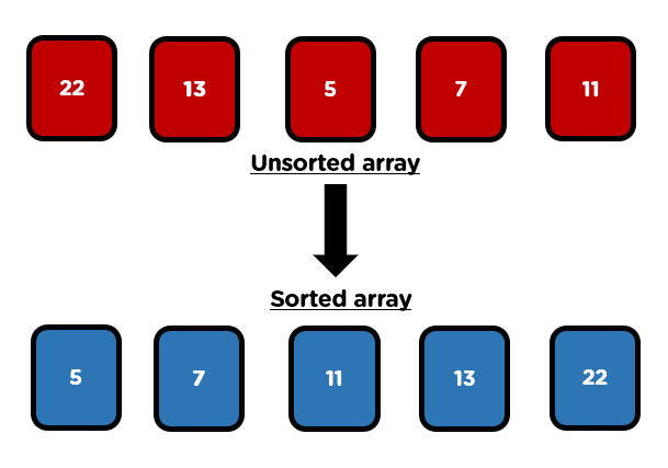

Sorting is the process of arranging data in a specific order, typically:
- Ascending order (small → large)
- Descending order (large → small)
Sorting is a fundamental operation in computer science and plays a crucial role in:
- Searching algorithms
- Data analysis
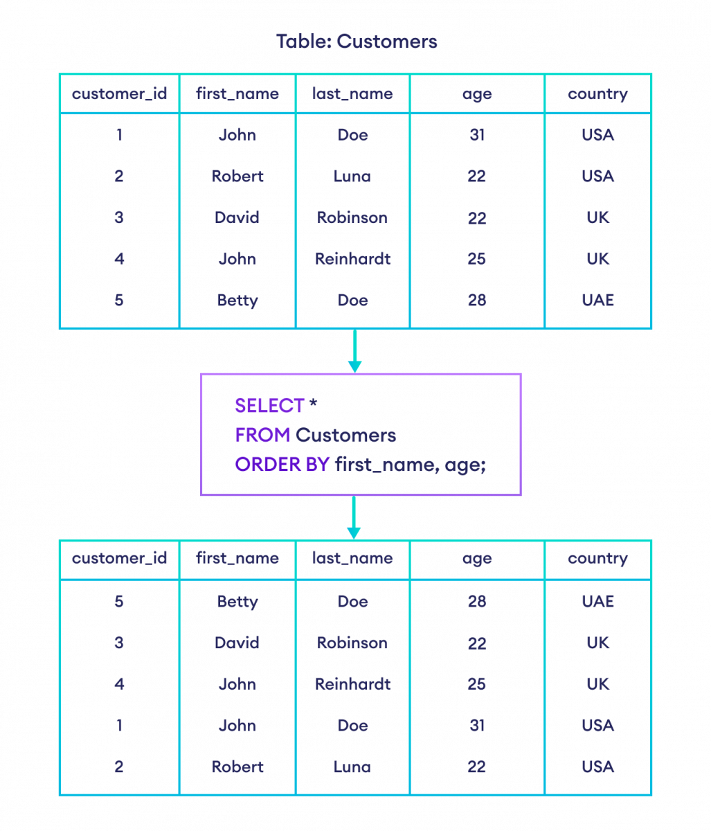
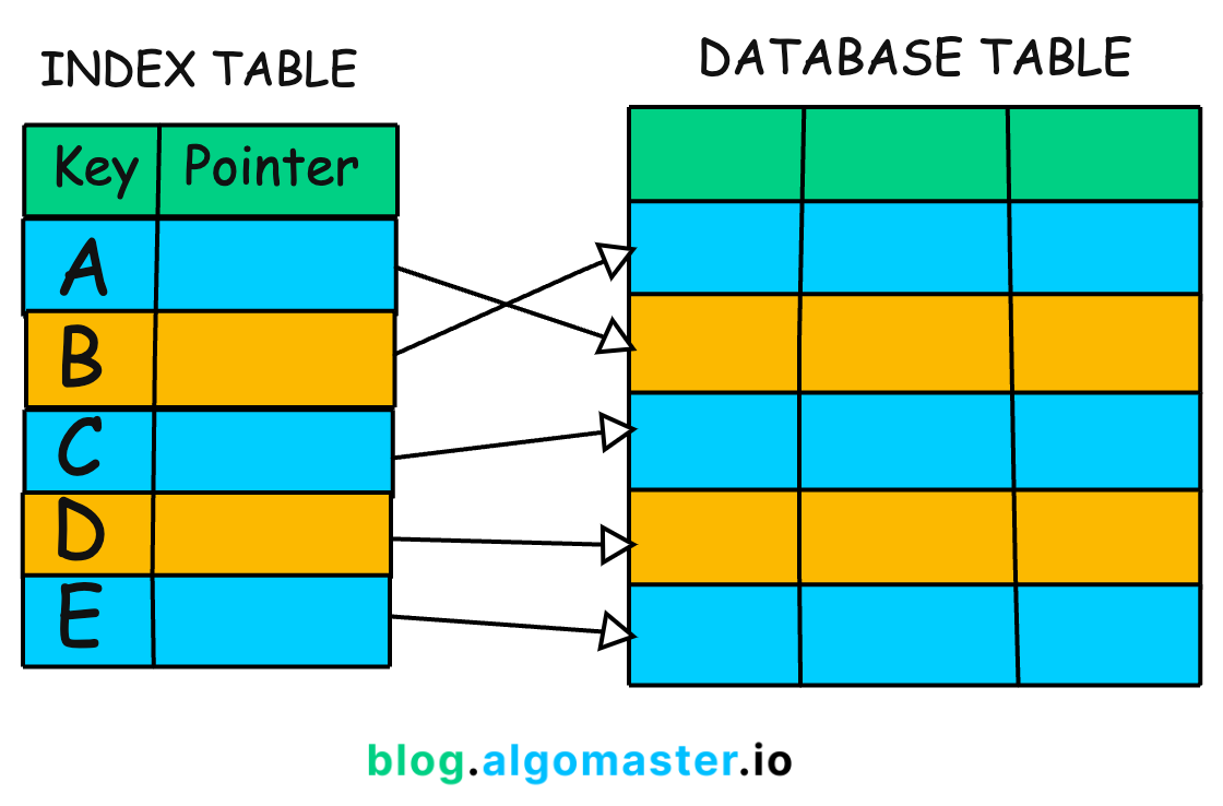
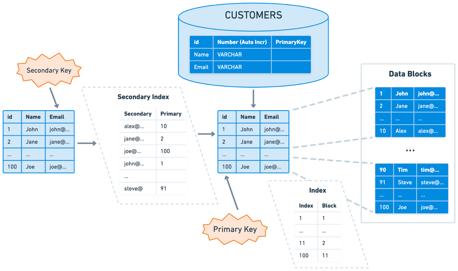
- Database management
- Optimization problems
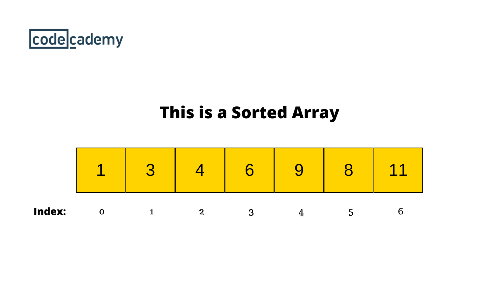
Example:
Unsorted: [5, 2, 9, 1, 6]
Sorted:   [1, 2, 5, 6, 9]
🧠 Why Sorting is Important
- Improves efficiency of searching (e.g., Binary Search)
- Enables easier data analysis
- Helps in duplicate detection
- Forms the backbone of many algorithms
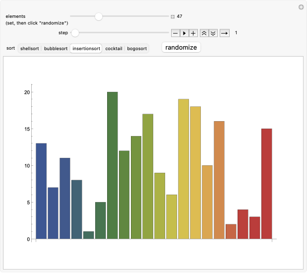
⚙️ Classification of Sorting Algorithms
Sorting algorithms can be classified based on several criteria:
🔹 Based on Method
- Comparison-based sorting
- Non-comparison-based sorting
🔹 Based on Memory Usage
- In-place sorting
- Out-of-place sorting
🔹 Based on Stability
- Stable sorting
- Unstable sorting
🔢 Comparison-Based Sorting Algorithms
🔹 1. Bubble Sort
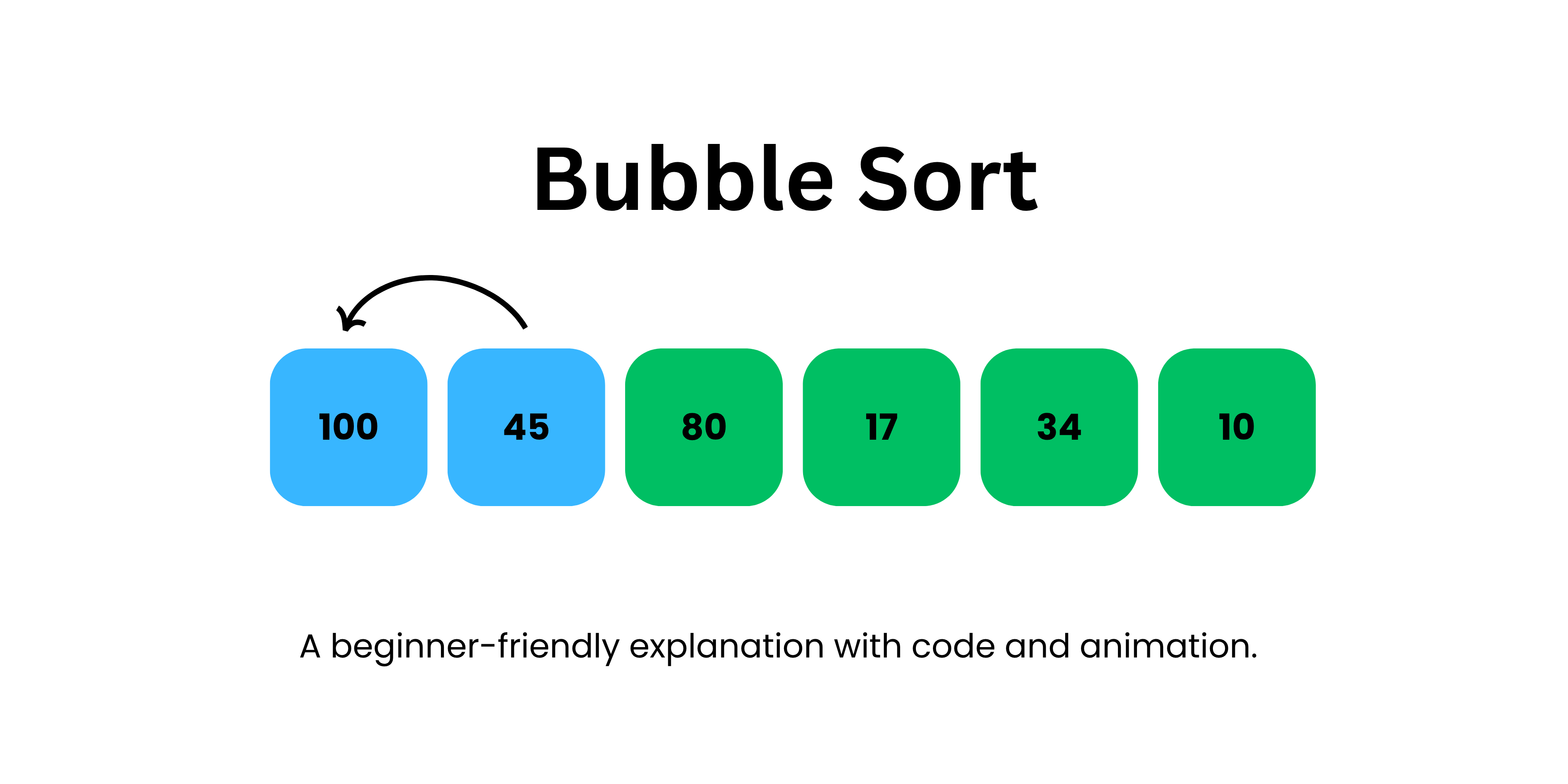
📌 Concept:
Repeatedly compares adjacent elements and swaps them if they are in the wrong order.
🧾 Algorithm:
- Compare adjacent elements
- Swap if needed
- Repeat until sorted
💻 Example:
def bubble_sort(arr):
n = len(arr)
for i in range(n):
for j in range(0, n-i-1):
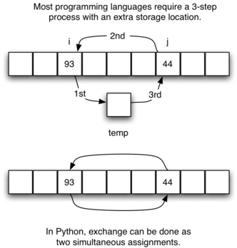
if arr[j] > arr[j+1]:
arr[j], arr[j+1] = arr[j+1], arr[j]
⏱️ Complexity:
- Best: O(n)
- Average: O(n²)
- Worst: O(n²)
✅ Pros:
- Simple
- Easy to understand
❌ Cons:
- Very slow for large data
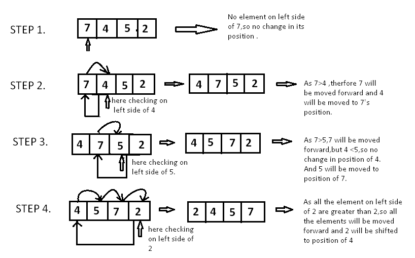
🔹 2. Selection Sort
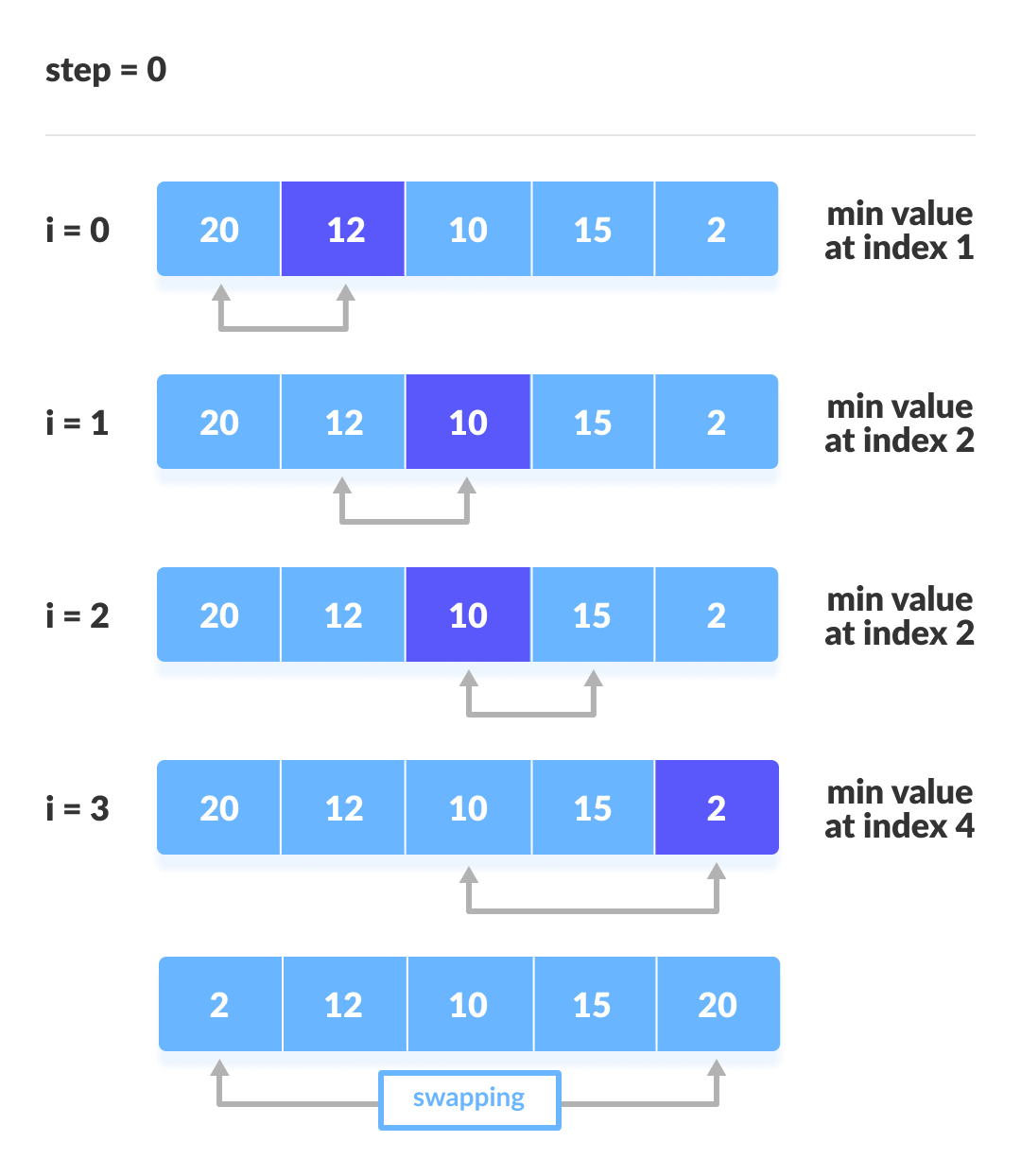
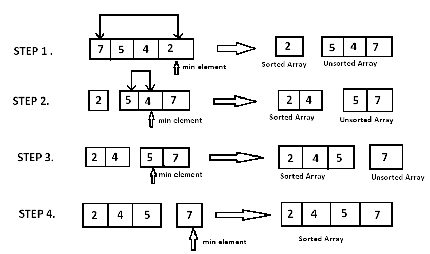
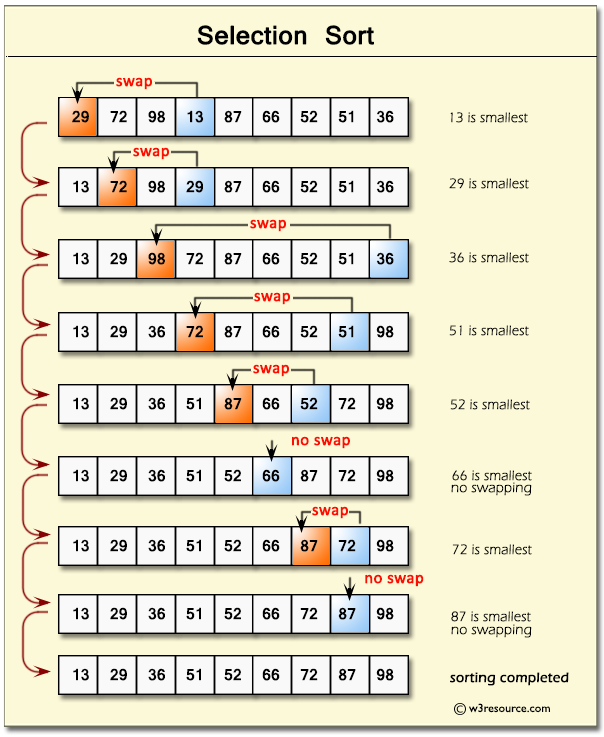
📌 Concept:
Selects the smallest element and places it in correct position.
⏱️ Complexity:
- O(n²) for all cases
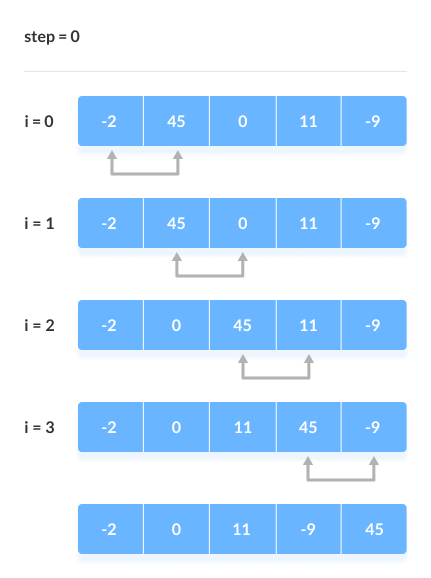
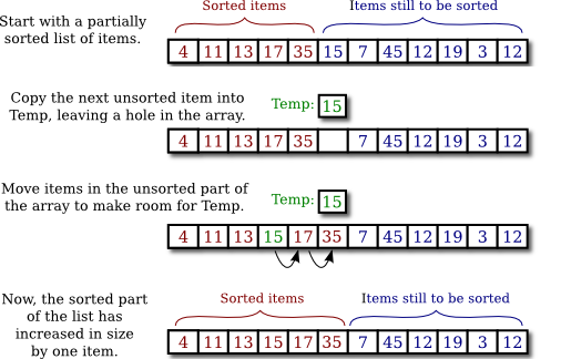
🔹 3. Insertion Sort

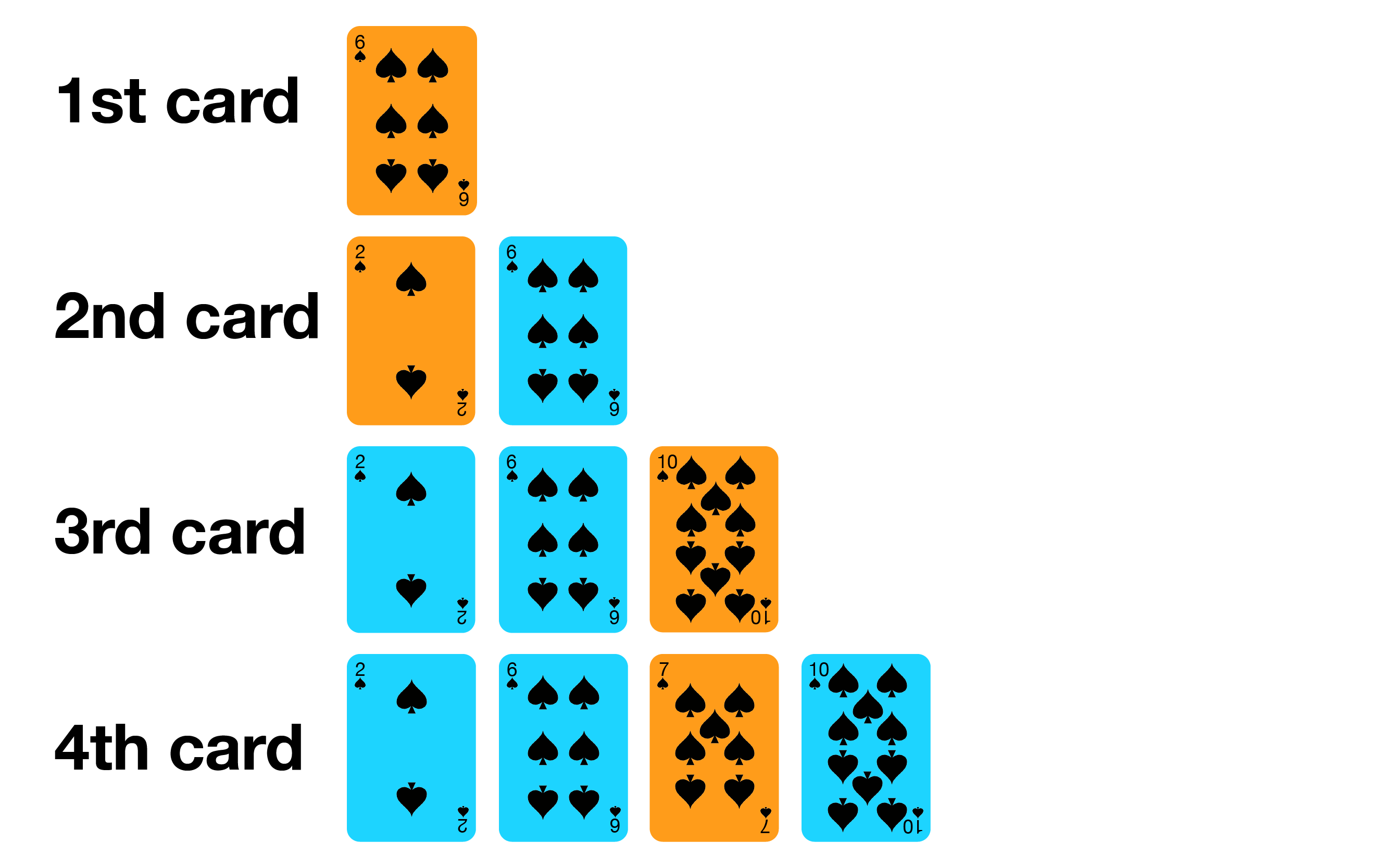
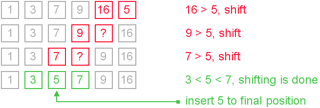
📌 Concept:
Builds sorted array one element at a time.
⏱️ Complexity:
- Best: O(n)
- Worst: O(n²)
📌 Use Case:
Small datasets
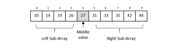
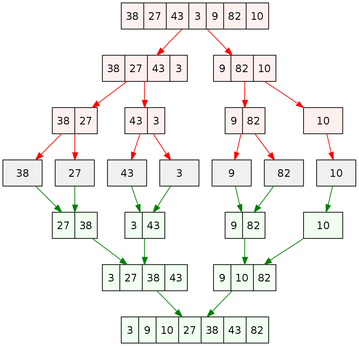
🔹 4. Merge Sort
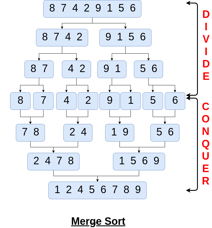
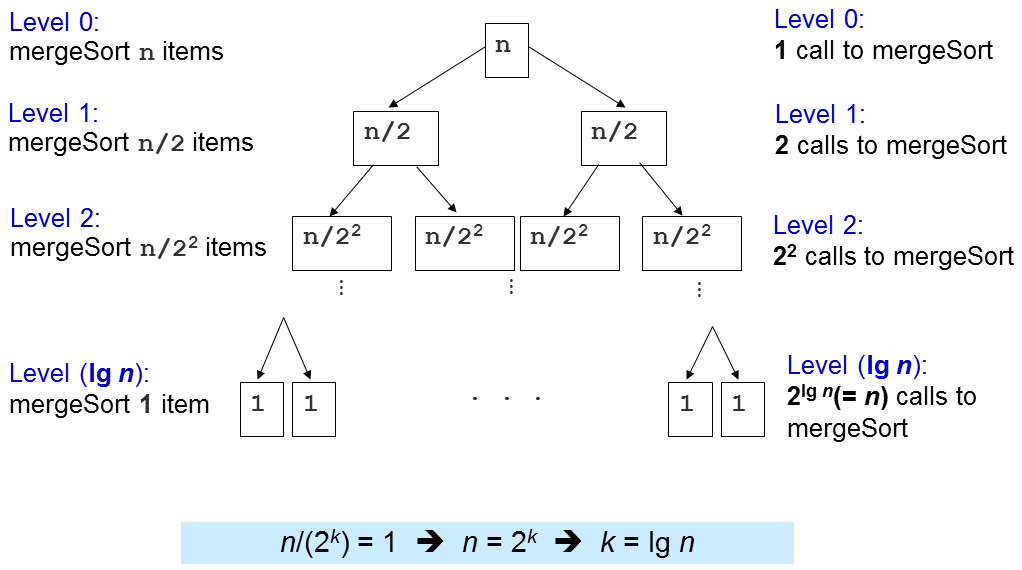
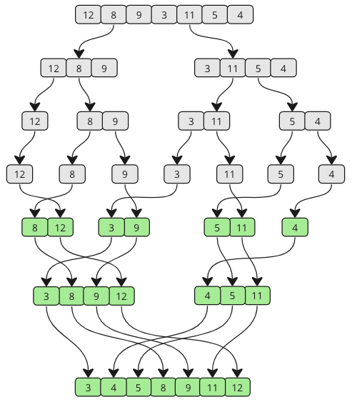
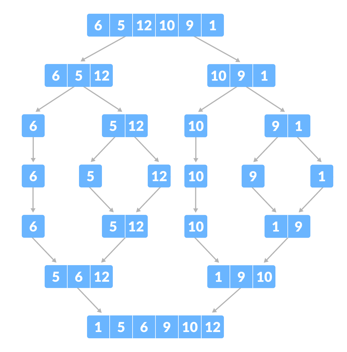
📌 Concept:
Divide and conquer algorithm.
Steps:
- Divide array into halves
- Sort each half
- Merge them
⏱️ Complexity:
- O(n log n)
✅ Pros:
- Stable
- Efficient
❌ Cons:
- Extra memory needed
🔹 5. Quick Sort

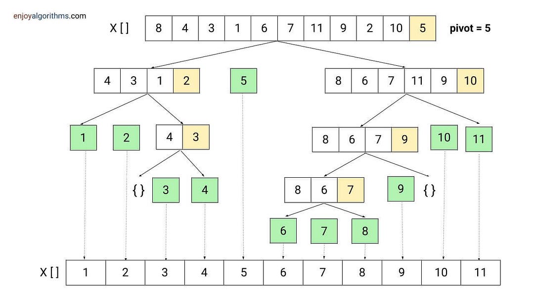
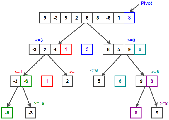

📌 Concept:
Uses pivot to partition array.
⏱️ Complexity:
- Best: O(n log n)
- Worst: O(n²)
✅ Pros:
- Fast in practice
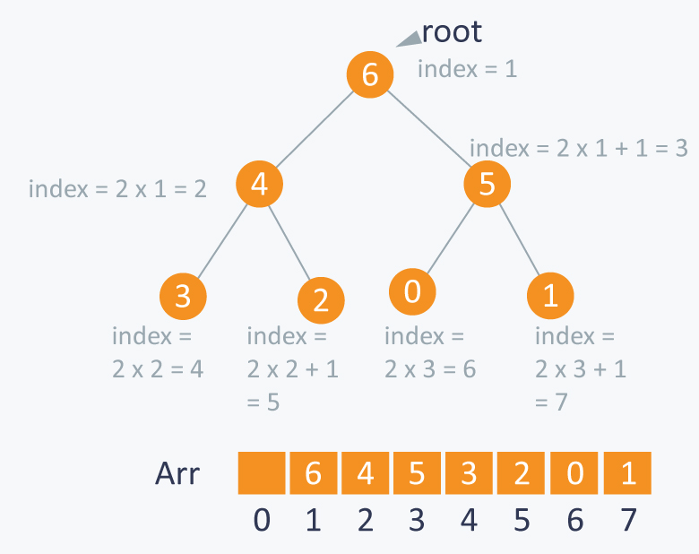
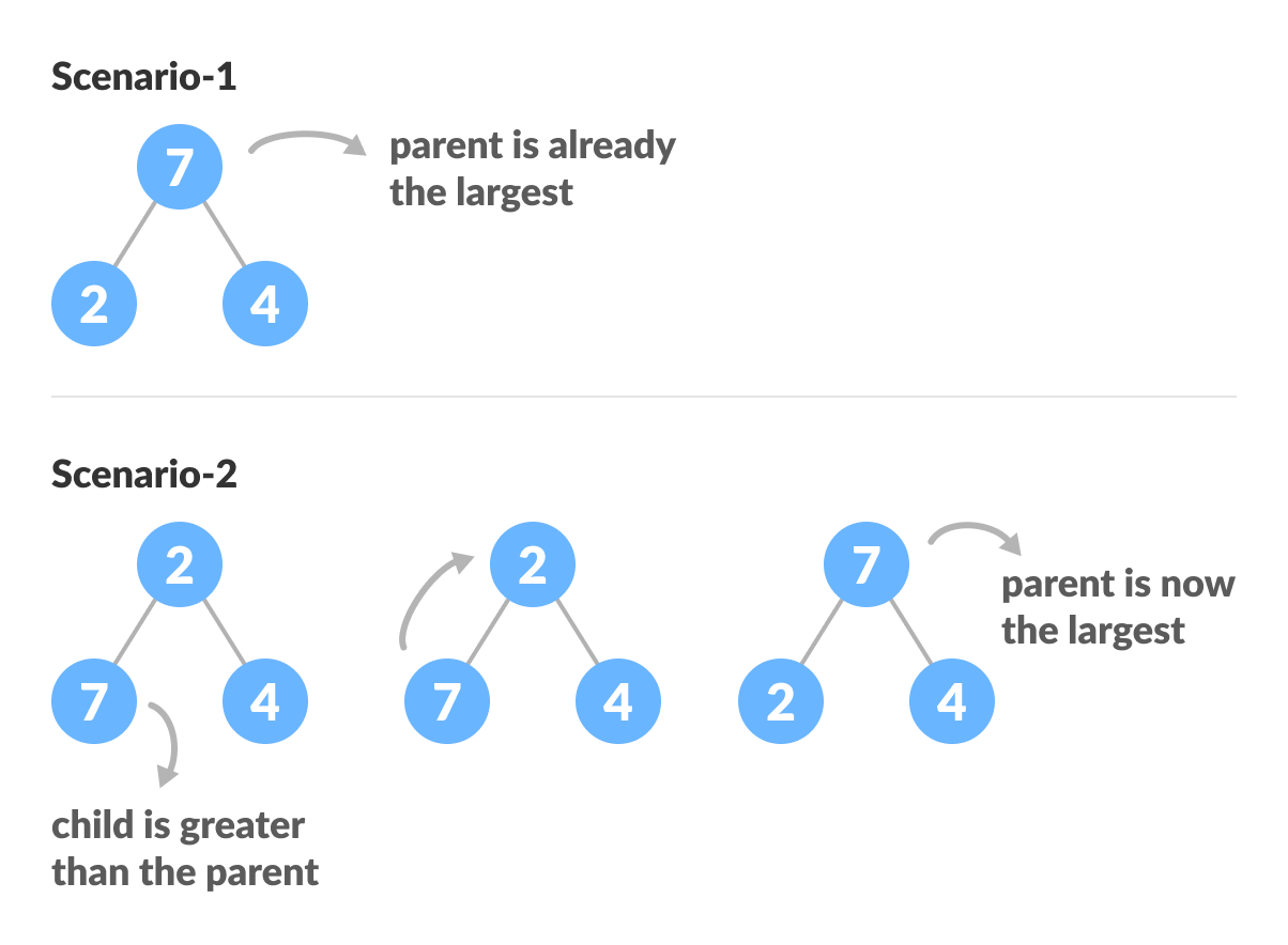
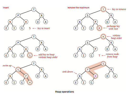
🔹 6. Heap Sort
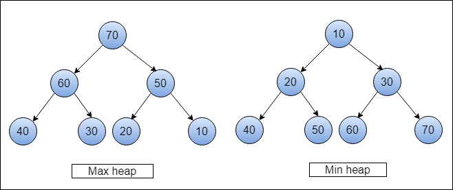

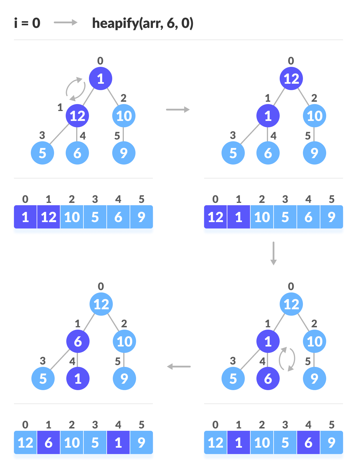
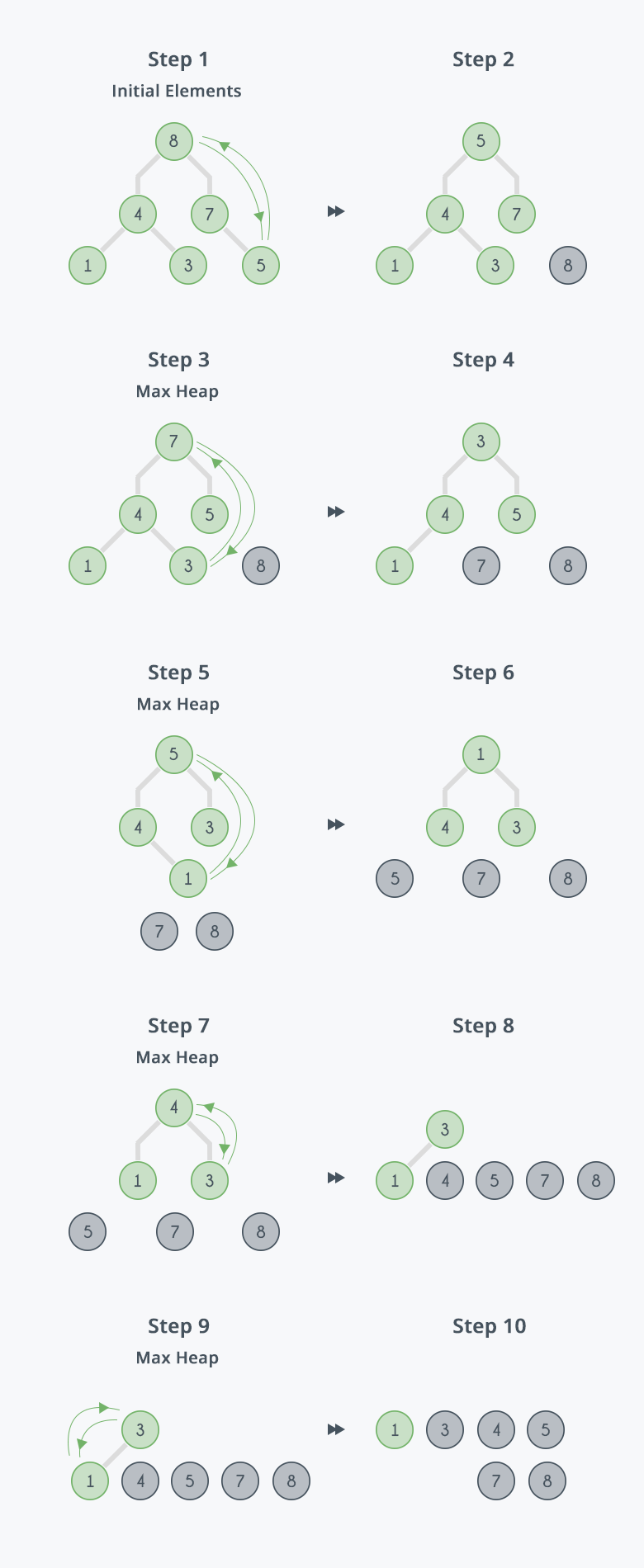
📌 Concept:
Uses binary heap.
⏱️ Complexity:
- O(n log n)
🔢 Non-Comparison Sorting Algorithms
🔹 1. Counting Sort
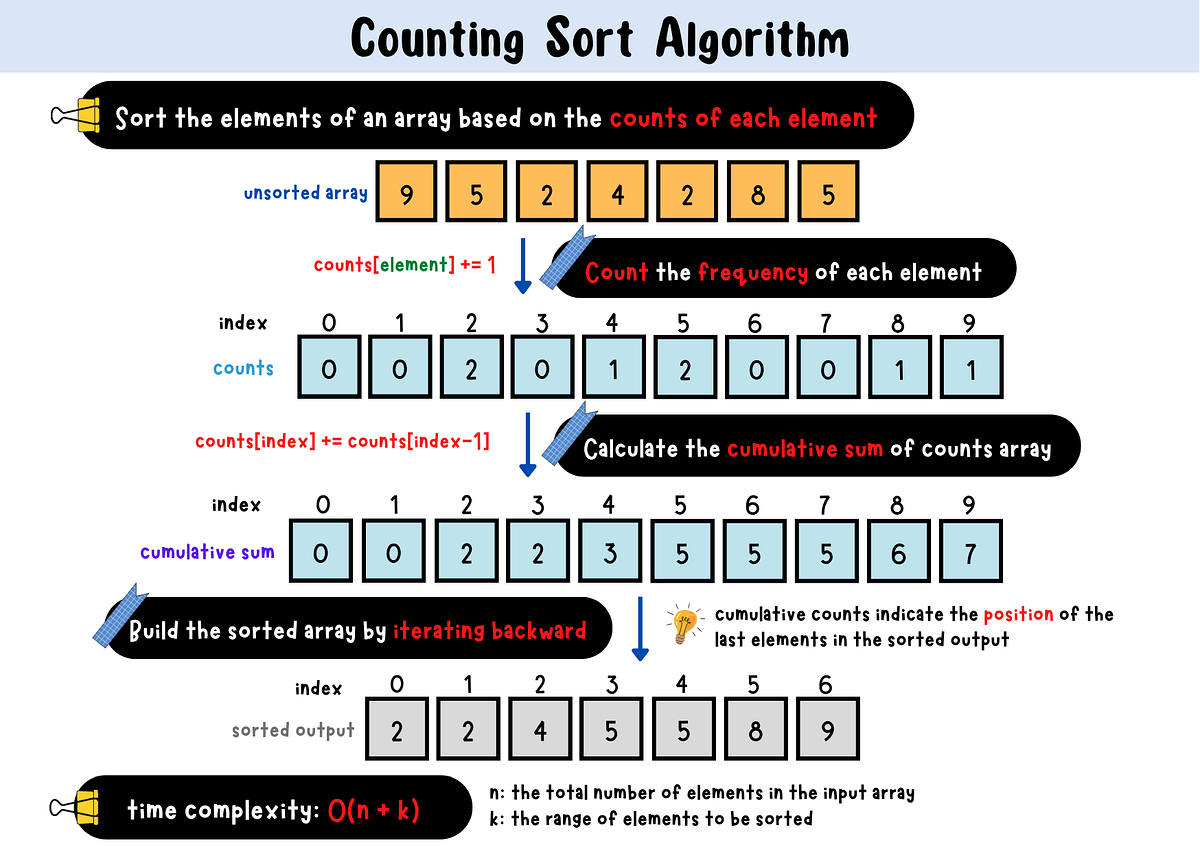
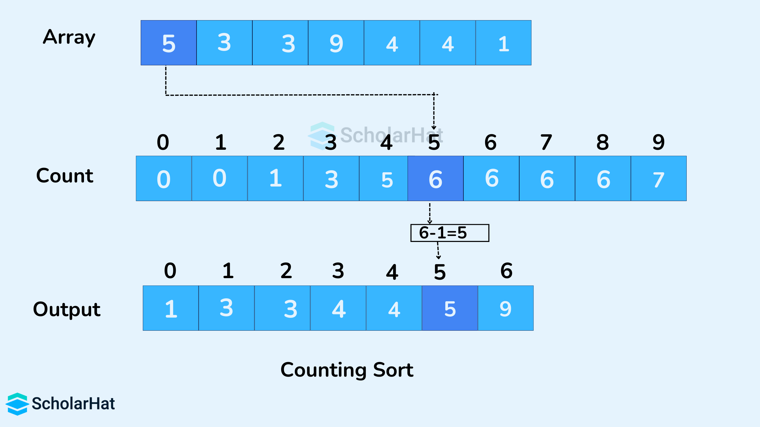
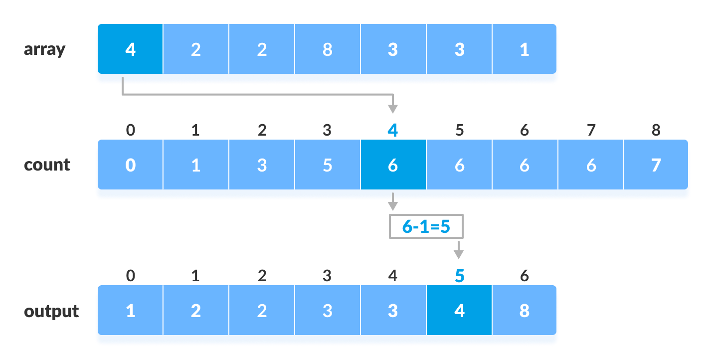
📌 Concept:
Counts occurrences of elements.
⏱️ Complexity:
- O(n + k)
🔹 2. Radix Sort


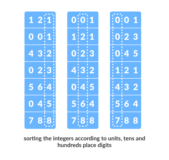
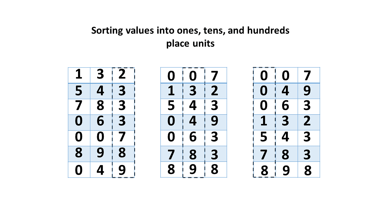
📌 Concept:
Sorts digits from least to most significant.
🔹 3. Bucket Sort

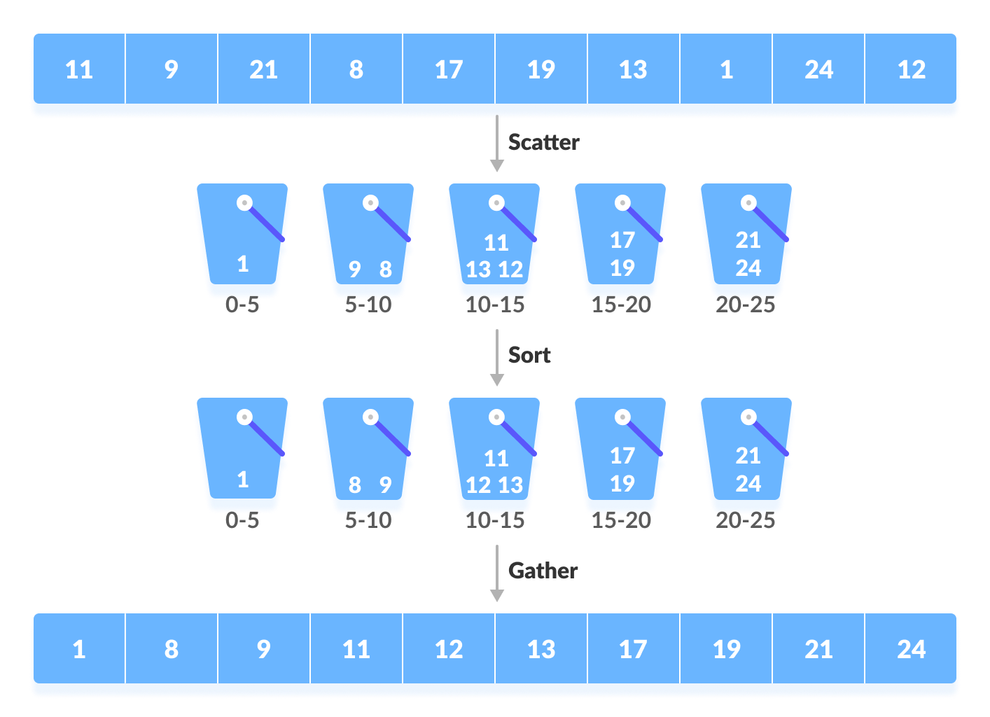

📌 Concept:
Distributes elements into buckets.
🧮 Time Complexity Comparison Table
| Algorithm | Best Case | Average | Worst Case |
|---|---|---|---|
| Bubble Sort | O(n) | O(n²) | O(n²) |
| Selection Sort | O(n²) | O(n²) | O(n²) |
| Insertion Sort | O(n) | O(n²) | O(n²) |
| Merge Sort | O(n log n) | O(n log n) | O(n log n) |
| Quick Sort | O(n log n) | O(n log n) | O(n²) |
| Heap Sort | O(n log n) | O(n log n) | O(n log n) |
| Counting Sort | O(n+k) | O(n+k) | O(n+k) |
| Radix Sort | O(nk) | O(nk) | O(nk) |
⚡ Stable vs Unstable Sorting
Stable Sorting:
Maintains order of equal elements.
- Merge Sort
- Insertion Sort
Unstable Sorting:
Does not preserve order.
- Quick Sort
- Heap Sort
🧠 Advanced Sorting Concepts
🔹 1. External Sorting


Used for data that doesn’t fit in memory.
🔹 2. Tim Sort
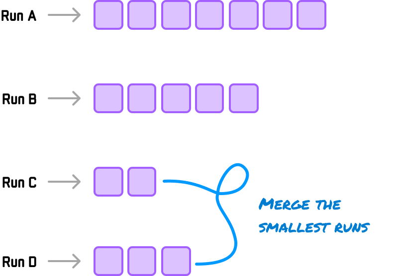


Hybrid of merge and insertion sort.
🔹 3. Intro Sort

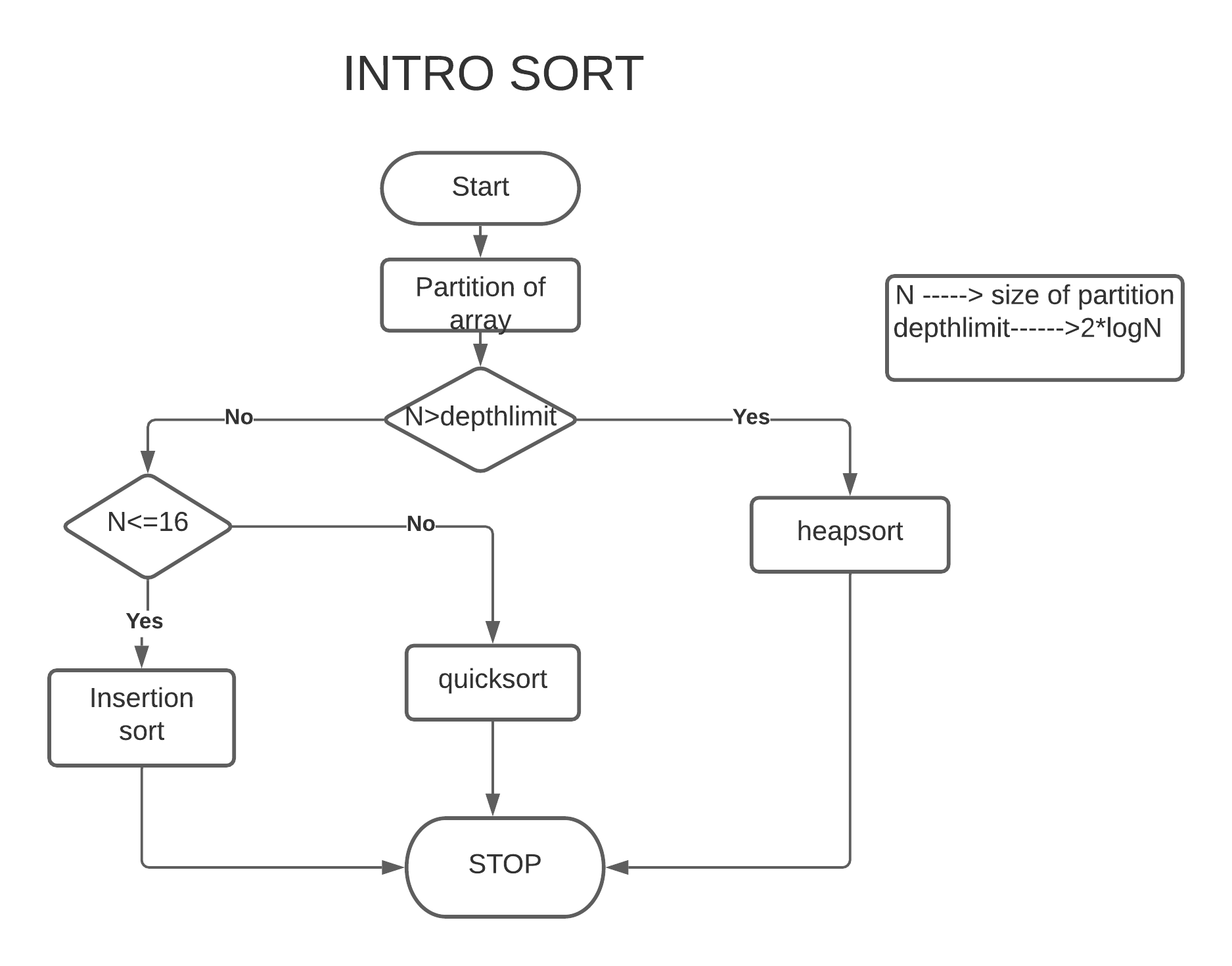


Combines Quick + Heap sort.
🔬 Applications of Sorting
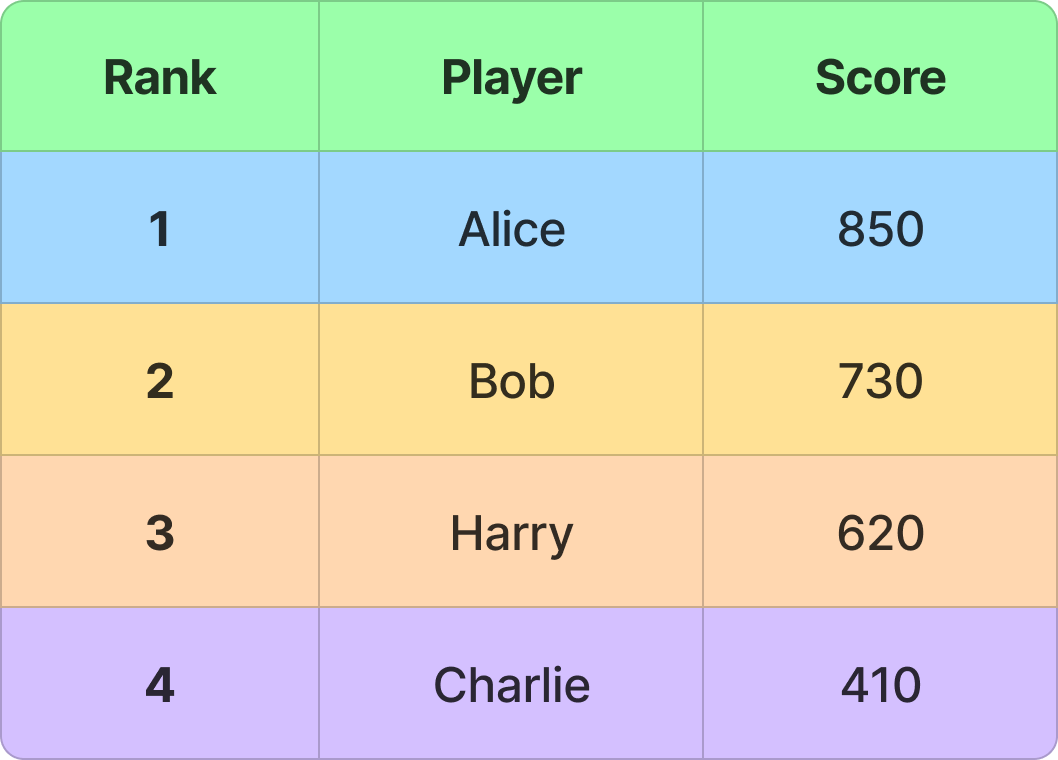
📊 1. Data Analysis


🌐 2. Search Optimization


🧾 3. Database Systems

🎮 4. Game Development

🧠 5. Machine Learning

🔁 Choosing the Right Algorithm
| Scenario | Best Algorithm |
|---|---|
| Small data | Insertion Sort |
| Large data | Merge / Quick Sort |
| Memory limited | Heap Sort |
| Integer range small | Counting Sort |
🧪 In-Place vs Out-of-Place
- In-place: Quick Sort, Heap Sort
- Out-of-place: Merge Sort
🚀 Real-World Importance
Sorting is used in:
- Operating systems
- Databases
- AI systems
- Web applications
- Financial systems
🧾 Conclusion
Sorting algorithms are essential tools in computer science that enable efficient data organization and processing. Each algorithm has its strengths and weaknesses, and choosing the right one depends on the specific problem.
Mastering sorting algorithms is crucial for:
- Algorithm design
- Competitive programming
- Software engineering